library(sf)           # Simple Features in R
library(terra)        # Raster Data in R
library(spData)       # Spatial Datasets
library(spDataLarge)  # Large Spatial Datasets
library(tidyverse) # Data Wrangling and VisualizationChapter 2: Geographic data in R
Key Learnings from, and Solutions to the exercises in Chapter 2 of the book Geocomputation with R by Robin Lovelace, Jakub Nowosad and Jannes Muenchow.
Geocomputation with R
Textbook Solutions
2.1 Introduction
- Geographic Data Models: Vector and raster models are foundational.
- Vector Model: Represents geographic data as points, lines, and polygons with precise boundaries; commonly used in social sciences for features like human settlements.
- Raster Model: Divides surfaces into cells; useful in environmental sciences, often based on remote sensing and aerial data. Scalable and consistent over large areas.
- Choosing a Model:
- Vector is often used in social sciences.
- Raster is prevalent in environmental studies.
- R Implementation:
2.2 Vector Data
- Vector Data: Represents geographic features using points, lines, and polygons based on coordinate reference systems (CRS).
- Example: London’s coordinates
c(-0.1, 51.5)in geographic CRS orc(530000, 180000)in projected CRS (British National Grid).
- Example: London’s coordinates
- CRS Overview:
- Geographic CRS uses
lon/lat(0° longitude and latitude origin). - Projected CRS, like the British National Grid, is based on
Easting/Northingcoordinates with positive values.
- Geographic CRS uses
- Key dependencies / libraries used by the
sfPackage: - Geometry Engines:
- Planar (GEOS): For 2D projected data.
- Spherical (S2): For 3D unprojected data.
2.2.1 Introduction to Simple Features
- Simple Features (SF): Hierarchical model by OGC (Open Geospatial Consortium); supports multiple geometry types.
- Core Types:
sfpackage in R supports 7 core geometry types (points, lines, polygons, and their “multi” versions). - Library Integration:
sfreplacessp,rgdal,rgeos; unified interface for GEOS (geometry), GDAL (data I/O), PROJ (CRS). - Non-Planar Support: Integrates
s2for geographic (lon/lat) operations, used by default for accuracy on spherical geometries. - Data Storage: SF objects are data frames with a spatial column (
geometryorgeom). - Vignettes: Documentation accessible with
vignette(package = "sf")for practical use and examples. - Plotting:
plot(sf_object)maps all variables, unlike single-map GIS tools. - Summary:
summary()gives spatial and attribute data insights. - Subset: SF objects subsettable like data frames, retaining spatial metadata.
worldSimple feature collection with 177 features and 10 fields
Geometry type: MULTIPOLYGON
Dimension: XY
Bounding box: xmin: -180 ymin: -89.9 xmax: 180 ymax: 83.64513
Geodetic CRS: WGS 84
# A tibble: 177 × 11
iso_a2 name_long continent region_un subregion type area_km2 pop lifeExp
* <chr> <chr> <chr> <chr> <chr> <chr> <dbl> <dbl> <dbl>
1 FJ Fiji Oceania Oceania Melanesia Sove… 1.93e4 8.86e5 70.0
2 TZ Tanzania Africa Africa Eastern … Sove… 9.33e5 5.22e7 64.2
3 EH Western … Africa Africa Northern… Inde… 9.63e4 NA NA
4 CA Canada North Am… Americas Northern… Sove… 1.00e7 3.55e7 82.0
5 US United S… North Am… Americas Northern… Coun… 9.51e6 3.19e8 78.8
6 KZ Kazakhst… Asia Asia Central … Sove… 2.73e6 1.73e7 71.6
7 UZ Uzbekist… Asia Asia Central … Sove… 4.61e5 3.08e7 71.0
8 PG Papua Ne… Oceania Oceania Melanesia Sove… 4.65e5 7.76e6 65.2
9 ID Indonesia Asia Asia South-Ea… Sove… 1.82e6 2.55e8 68.9
10 AR Argentina South Am… Americas South Am… Sove… 2.78e6 4.30e7 76.3
# ℹ 167 more rows
# ℹ 2 more variables: gdpPercap <dbl>, geom <MULTIPOLYGON [°]>names(world) [1] "iso_a2" "name_long" "continent" "region_un" "subregion" "type"
[7] "area_km2" "pop" "lifeExp" "gdpPercap" "geom" class(world)[1] "sf" "tbl_df" "tbl" "data.frame"########### THE GEOMETRY COLUMN IS STICKY ################
summary(world["lifeExp"]) lifeExp geom
Min. :50.62 MULTIPOLYGON :177
1st Qu.:64.96 epsg:4326 : 0
Median :72.87 +proj=long...: 0
Mean :70.85
3rd Qu.:76.78
Max. :83.59
NA's :10 Code
plot(world)
2.2.2 Why Simple Features?
- Cross-Compatibility: SF model is compatible with many GIS tools (e.g., QGIS, PostGIS), enabling easy data transfer.
- Advantages of
sfinR:- Data Handling: Fast reading/writing of spatial data.
- Plotting: Improved plotting speed and performance.
- Data Frame-Like:
sfobjects behave like data frames. - Consistent Naming:
sffunctions are intuitive, starting withst_. - Tidyverse-Friendly: Works well with
|>and integrates with tidyverse packages.
- Data Import Options:
read_sf(): Imports data as a tidy tibble (quietly).st_read(): Imports data as a base R data frame (verbose).
- Popularity:
sfis the primary package for spatial vector data in R, preferred over alternatives likespatstatandterra.
world_dfr <- st_read(system.file("shapes/world.shp", package = "spData"))
## Reading layer `world' from data source
##   `C:\Users\dradi\AppData\Local\R\win-library\4.3\spData\shapes\world.shp'
##   using driver `ESRI Shapefile'
## Simple feature collection with 177 features and 10 fields
## Geometry type: MULTIPOLYGON
## Dimension:     XY
## Bounding box:  xmin: -180 ymin: -89.9 xmax: 180 ymax: 83.64513
## Geodetic CRS:  WGS 84
world_dfr <- read_sf(system.file("shapes/world.shp", package = "spData"))

class(world_dfr)
## [1] "sf"         "tbl_df"     "tbl"        "data.frame"
2.2.3 Basic Maps
- Plotting in
sf:plot()creates multi-panel plots for multiple variables or a single-panel plot for one variable.- Supports fixed color customization using
colandborderarguments.
Code
plot(world)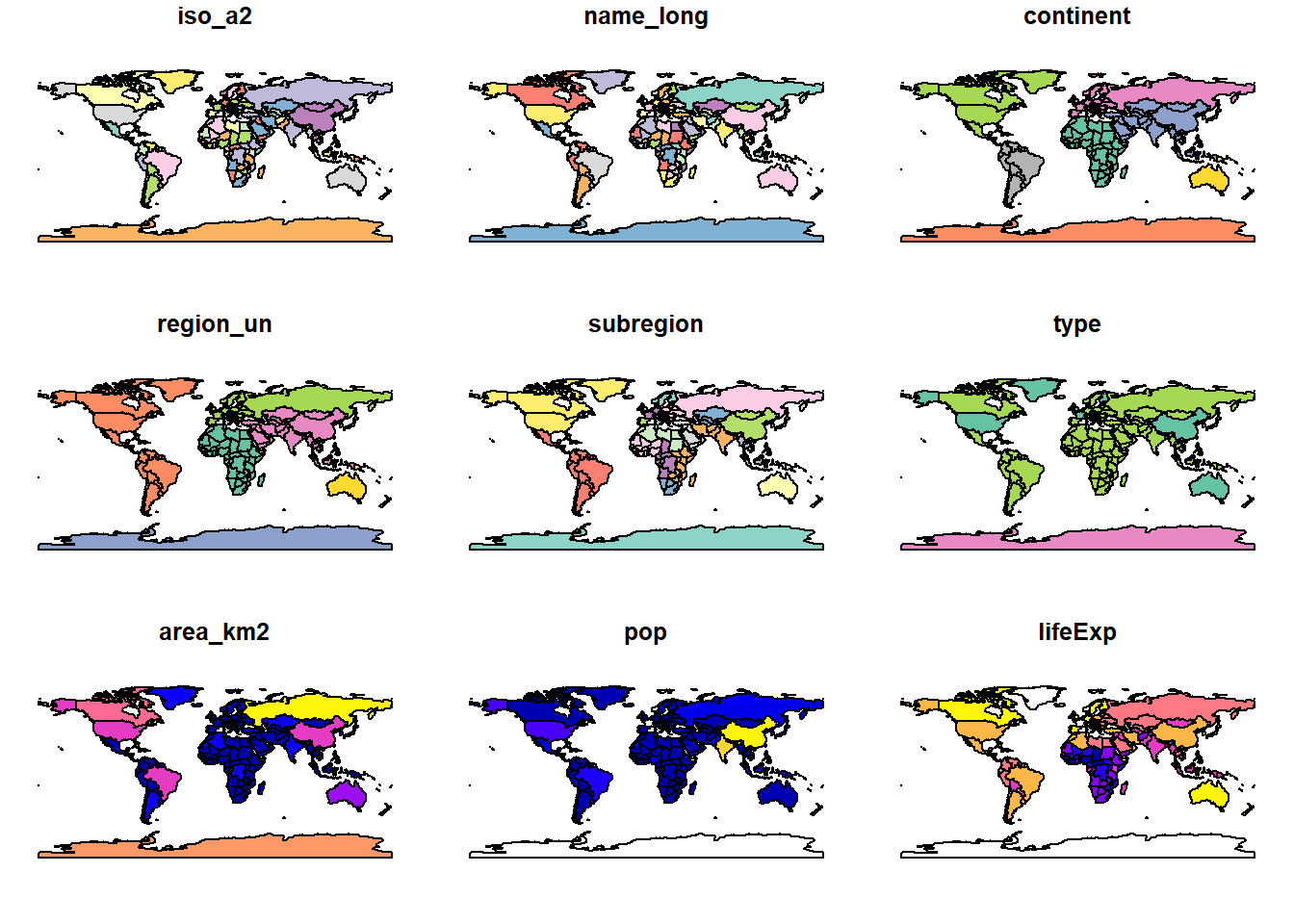
- Layering Plots: Add layers to existing plots with
add = TRUE. Usereset = FALSEfor plots with a key. - Overlaying Data: Circles representing population size can be plotted using
cexandst_centroid(). - Bounding Box Expansion:
expandBBadjusts the plot boundaries (bottom, left, top, right). - Limitations: Base
plot()is simple but limited in functionality; usetmapfor advanced maps.
2.2.4 Geometry Types
- Geometry Basics:
- Core components of simple features;
sfsupports 18 types. - Focus on 7 common types: POINT, LINESTRING, POLYGON, MULTIPOINT, MULTILINESTRING, MULTIPOLYGON, GEOMETRYCOLLECTION.
- Core components of simple features;
- Encoding Standards:
- WKB (Well-known binary): Hexadecimal, computer-friendly format.
- WKT (Well-known text): Human-readable format, often shown for explanation.
- Common Geometries:
- POINT: Single coordinate (e.g.,
POINT (5 2)). - LINESTRING: Connected sequence of points (e.g.,
LINESTRING (1 5, 4 4, 4 1, 2 2, 3 2)). - POLYGON: Closed ring of points (e.g.,
POLYGON ((1 5, 2 2, 4 1, 4 4, 1 5))).
- POINT: Single coordinate (e.g.,
- Multi-Geometries:
- MULTIPOINT: Multiple points (e.g.,
MULTIPOINT (5 2, 1 3, 3 4, 3 2)). - MULTILINESTRING: Multiple linestrings (e.g.,
MULTILINESTRING ((1 5, 4 4, 4 1, 2 2, 3 2), (1 2, 2 4))). - MULTIPOLYGON: Multiple polygons (e.g.,
MULTIPOLYGON (((1 5, 2 2, 4 1, 4 4, 1 5), (0 2, 1 2, 1 3, 0 3, 0 2)))).
- MULTIPOINT: Multiple points (e.g.,
- Geometry Collection:
- Mix of geometry types (e.g.,
GEOMETRYCOLLECTION (MULTIPOINT (5 2, 1 3, 3 4, 3 2), LINESTRING (1 5, 4 4, 4 1, 2 2, 3 2))).
- Mix of geometry types (e.g.,
2.2.5 The sf Class
Structure of sf Objects: Composed of geometries (
sfcobject) and non-geographic attributes (data.frameortibble).Creation of sf Objects: Steps:
Create geometry (
sfg) with functions likest_point()Convert to geometry column (
sfc) with CRS using functionst_sfc(..., crs = "...")Combine attributes (
data.frame) withsfcusing functionst_sf(..., geometry = ...)
Characteristics:
sfobjects have dual class:sfanddata.frame.- Spatial attributes stored in a
geometrycolumn. sfbehaves like adata.framebut with spatial extension.
2.2.6 Simple Feature Geometries (sfg)
An sfg object represents a single simple feature geometry. A simple feature geometry column (sfc) is a collection of sfg objects and can also include information about the coordinate reference system (CRS) being used.
Geometries can be created using st_ functions or imported from existing spatial files.
- sfg Creation Functions:
st_point(): Create a single point.st_linestring(): Create a linestring.st_polygon(): Create a polygon.st_multipoint(): Create a multipoint.st_multilinestring(): Create a multilinestring.st_multipolygon(): Create a multipolygon.st_geometrycollection(): Create a geometry collection.
- Input Data Types:
- Numeric Vector: Single points.
- Matrix: Sets of points for multipoint or linestring.
- List: Complex structures for multilinestrings, (multi)polygons, or geometry collections.
- Examples:
Code
# Create a point
point <- st_point(c(8, 3)) # POINT (8 3)
print(point)
ggplot(point) +
geom_sf()
# Create a multipoint
multipoint_matrix <- rbind(c(8, 3), c(2, 5), c(5, 7), c(7, 3))
multipoint <- st_multipoint(multipoint_matrix) # MULTIPOINT ((8 3), (2 5), (5 7), (7 3))
print(multipoint)
ggplot(multipoint) +
geom_sf()
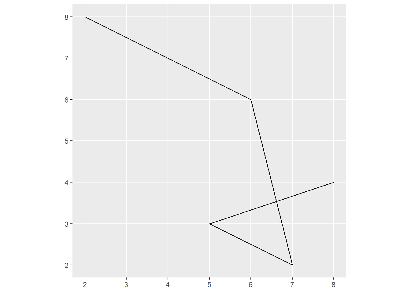
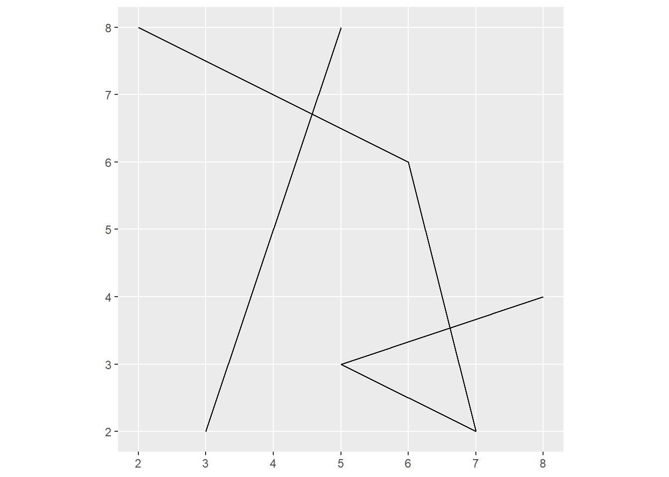
# Create a linestring
linestring_matrix <- rbind(c(2, 8), c(6, 6), c(7, 2), c(5, 3), c(8, 4))
linestring <- st_linestring(linestring_matrix) # LINESTRING (2 8, 6 6, 7 2, 5 3, 8 4)
print(linestring)
ggplot(linestring) +
geom_sf()
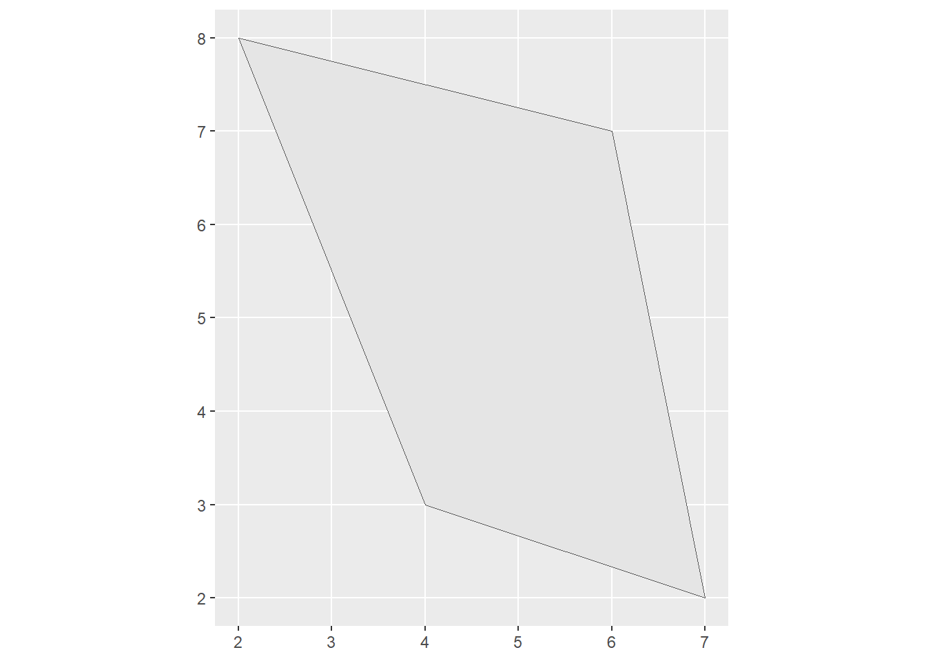
# Create a polygon
polygon_list <- list(rbind(c(2, 8), c(4, 3), c(7, 2), c(6, 7), c(2, 8)))
polygon <- st_polygon(polygon_list) # POLYGON ((2 8, 4 3, 7 2, 6 7, 2 8))
print(polygon)
ggplot(polygon) +
geom_sf()
# Polygon with a hole
polygon_border <- rbind(c(2, 8), c(4, 3), c(7, 2), c(6, 7), c(2, 8))
polygon_hole <- rbind(c(4, 6), c(5, 6), c(5, 5), c(4, 5), c(4, 6))
polygon_with_hole_list <- list(polygon_border, polygon_hole)
polygon_with_hole <- st_polygon(polygon_with_hole_list) # POLYGON with a hole
print(polygon_with_hole)
ggplot(polygon_with_hole) +
geom_sf()
# Create a multilinestring
multilinestring_list = list(
rbind(c(2, 8), c(6, 6), c(7, 2), c(5, 3), c(8, 4)),
rbind(c(3, 2), c(5, 8))
)
multilinestring = st_multilinestring(multilinestring_list) # MULTILINESTRING
print(multilinestring)
ggplot(multilinestring) +
geom_sf()
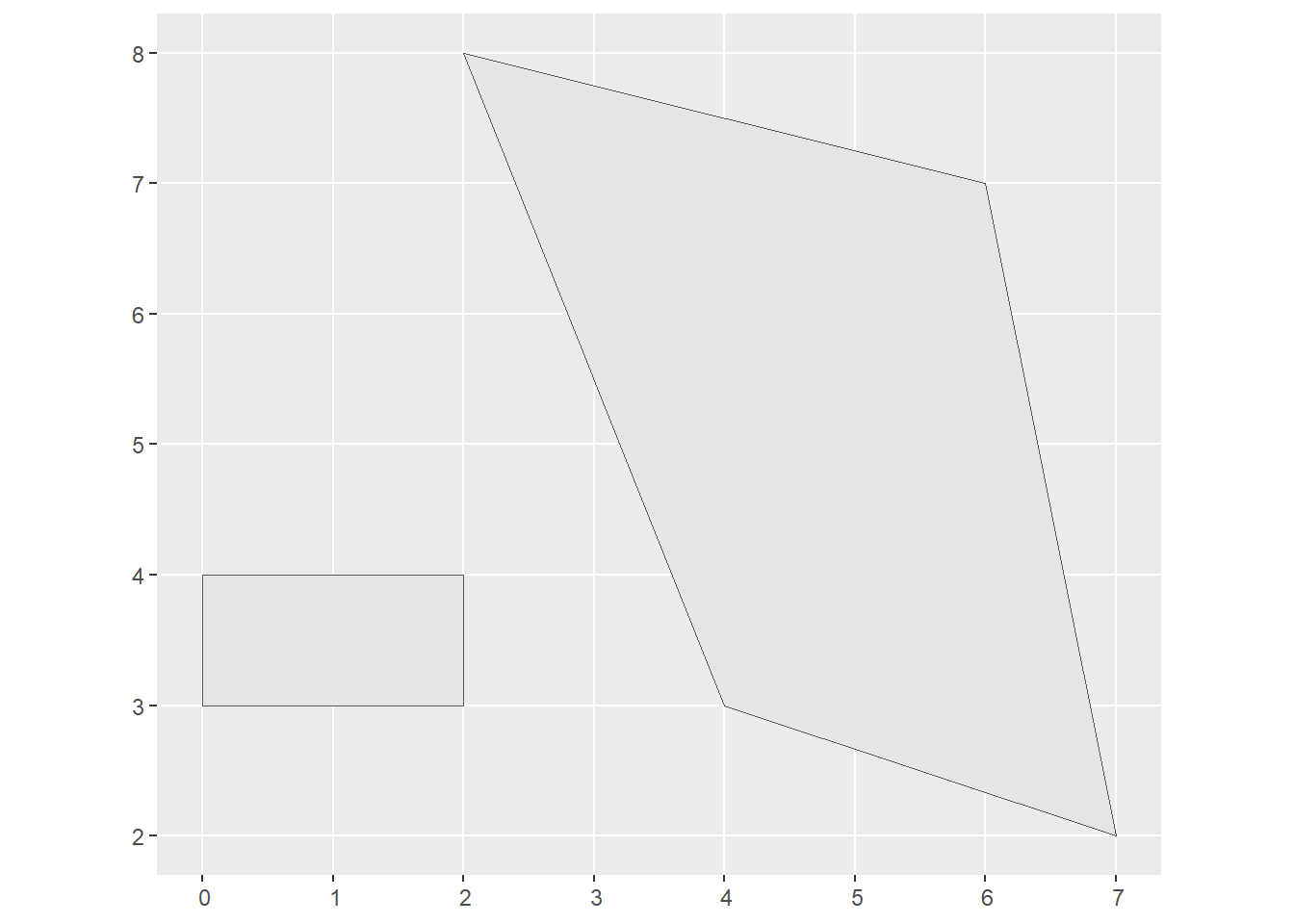
# Create a multipolygon
multipolygon_list = list(
list(rbind(c(2, 8), c(4, 3), c(7, 2), c(6, 7), c(2, 8))),
list(rbind(c(0, 3), c(2, 3), c(2, 4), c(0, 4), c(0, 3)))
)
multipolygon = st_multipolygon(multipolygon_list) # MULTIPOLYGON
print(multipolygon)
ggplot(multipolygon) +
geom_sf()
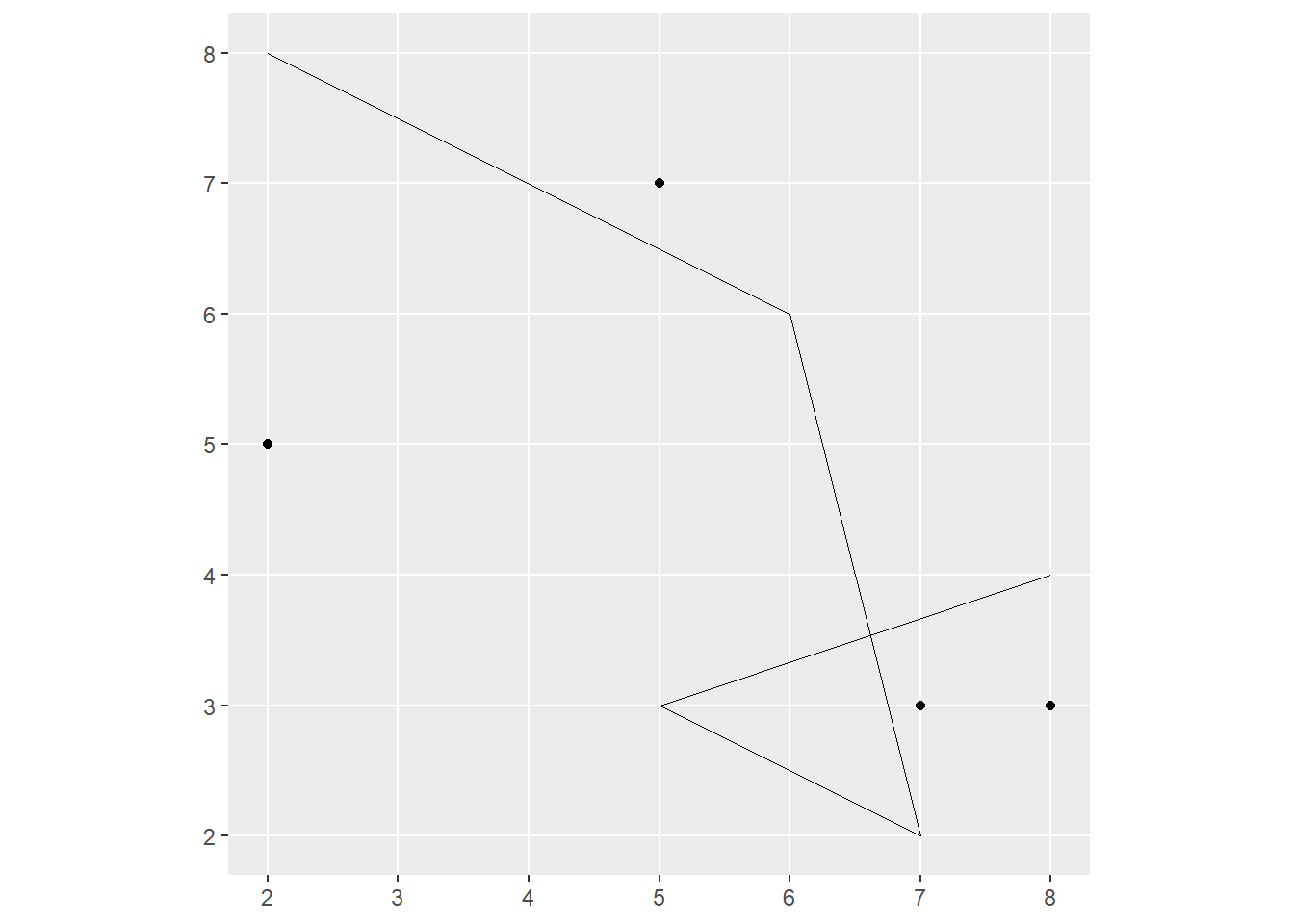
# Create a geometry collection
geometrycollection_list = list(st_multipoint(multipoint_matrix), st_linestring(linestring_matrix))
geometry_collection = st_geometrycollection(geometrycollection_list) # GEOMETRYCOLLECTION
print(geometry_collection)
ggplot(geometry_collection) +
geom_sf()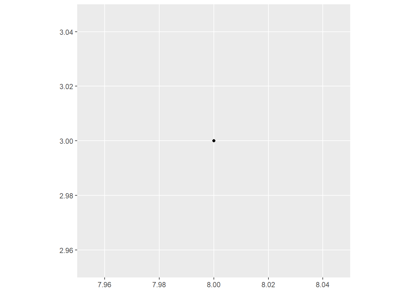


2.2.8 The sfheaders Package
- Overview:
sfheaders(Cooley 2024) is an R package designed to efficiently create and manipulatesfobjects from vectors, matrices, and data frames.- It does not rely on the
sflibrary and instead uses underlying C++ code, enabling faster operations and the potential for further development with compiled code.
- Compatibility:
- Although separate from
sf, it is fully compatible, producing validsfobjects likesfg,sfc, andsf.
- Although separate from
- Key Functionality:
- Converts:
- Vector →
sfg_POINT - Matrix →
sfg_LINESTRING - Data Frame →
sfg_POLYGON
- Vector →
- Creates
sfcandsfobjects using similar syntax.
- Converts:
- Advantages:
sfheadersis optimized for high-speed ‘deconstruction’ and ‘reconstruction’ ofsfobjects and casting between geometry types, offering faster performance thansfin many cases.
2.2.9 Spherical Geometry Operations with S2
- Concept:
- Spherical geometry operations acknowledge Earth’s roundness, as opposed to planar operations that assume flat surfaces.
- Since
sfversion 1.0.0, R integrates with Google’s S2 spherical geometry engine, enabling accurate global spatial operations. - S2 supports operations like distance, buffer, and area calculations, allowing accurate geocomputation on a spherical Earth model.
- Known as a Discrete Global Grid System (DGGS), S2 is similar to other systems like H3, which is a global hexagonal index.
- S2 Mode:
By default, S2 is enabled in
sf. Verify with:sf_use_s2()Turning Off S2:
sf_use_s2(FALSE)
- S2 Limitations and Edge Cases:
- Some operations may fail due to S2’s stricter definitions, potentially affecting legacy code. Error messages such as
Error in s2_geography_from_wkb ...might require turning off S2.
- Some operations may fail due to S2’s stricter definitions, potentially affecting legacy code. Error messages such as
- Recommendation:
- Keep S2 enabled for accurate global calculations unless specific operations necessitate its deactivation.
2.3 Raster Data
- The raster data model represents the world as a continuous grid of cells (pixels). Focuses on regular grids, where each cell is of constant size, though other grid types (e.g., rotated, sheared) exist.
- Structure:
- Comprises a raster header and a matrix of equally spaced cells.
- The raster header includes:
- CRS (Coordinate Reference System)
- Extent (geographical area covered)
- Origin (starting point, often the lower left corner; the
terrapackage defaults to the upper left).
- Extent is defined by:
- Number of columns (ncol)
- Number of rows (nrow)
- Cell size resolution
- Cell Access and Modification:
- Cells can be accessed and modified by:
- Cell ID
- Explicitly specifying row and column indices.
- This matrix representation is efficient as it avoids storing corner coordinates (unlike vector polygons).
- Cells can be accessed and modified by:
- Data Characteristics:
- Each cell can hold a single value, which can be either:
- Continuous (e.g., elevation, temperature)
- Categorical (e.g., land cover classes).
- Each cell can hold a single value, which can be either:
- Applications:
- Raster maps are useful for continuous phenomena (e.g., temperature, population density) and can also represent discrete features (e.g., soil classes).
2.3.1 R Packages for Working with Raster Data
- Several R packages for reading and processing raster datasets have emerged over the last two decades. The
rasterpackage was the first significant advancement in R’s raster capabilities when launched in 2010. It was the premier package until the development ofterraandstars, both offering powerful functions for raster data. - This book emphasizes
terra, which replaces the older, slower raster package. - Comparison of
terraandstars:
| Feature | terra |
stars |
|---|---|---|
| Primary Focus | Regular grids | Supports regular, rotated, sheared, rectilinear, and curvilinear grids |
| Data Structure | One or multi-layered rasters | Raster data cubes with multiple layers, time steps, and attributes |
| Memory Management | Uses C++ code and pointers for data storage | Uses lists of arrays for smaller rasters; file paths for larger ones |
| Vector Data Integration | Uses its own class SpatVector but supports sf objects |
Closely related to vector objects/functions in sf |
| Functions & Methods | Large number of built-in, purpose-specific functions (e.g., re-sampling, cropping) | Mix of built-in functions (st_ prefix), existing dplyr functions, and custom methods for R functions |
| Conversion Between Packages | Conversion to stars with st_as_stars() |
Conversion to terra with rast() |
| Performance | Generally optimized for speed and memory efficiency | Flexible, but performance varies based on data type and structure |
| Best Use Cases | Single or multi-layer rasters; fast processing | Complex data cubes with layers over time and multiple attributes |
| Programming Language Basis | Primarily C++ | R with some C++ integration |
2.3.2 Introduction to terra
- The
terrapackage is designed for handling raster objects in R, supporting a range of functions to create, read, export, manipulate, and process raster datasets.- While its functionality is similar to the older
rasterpackage,terraoffers improved computational efficiency. - Despite
terra’s advantages, therasterclass system remains popular due to its widespread use in other R packages. terraprovides seamless translation between the two object types using functions likeraster(),stack(), andbrick()for backward compatibility.
- While its functionality is similar to the older
- Key Features:
- Low-Level Functionality: Includes functions that help in building new tools for raster data processing.
- Memory Management: Supports processing of large raster datasets by dividing them into smaller chunks for iterative processing, allowing operations beyond available RAM capacity.
Code
raster_filepath <- system.file("raster/srtm.tif",
                              package = "spDataLarge")
my_rast <- rast(raster_filepath)

class(my_rast)
## [1] "SpatRaster"
## attr(,"package")
## [1] "terra"

ext(my_rast)
## SpatExtent : -113.239583212784, -112.85208321281, 37.1320834298579, 37.5129167631658 (xmin, xmax, ymin, ymax)

print(my_rast)
## class       : SpatRaster
## dimensions  : 457, 465, 1  (nrow, ncol, nlyr)
## resolution  : 0.0008333333, 0.0008333333  (x, y)
## extent      : -113.2396, -112.8521, 37.13208, 37.51292  (xmin, xmax, ymin, ymax)
## coord. ref. : lon/lat WGS 84 (EPSG:4326)
## source      : srtm.tif
## name        : srtm
## min value   : 1024
## max value : 2892- Dedicated Reporting Functions:
dim(): Number of rows, columns, and layers.ncell(): Total number of cells (pixels).res(): Spatial resolution.ext(): Spatial extent.crs(): Coordinate reference system (CRS).inMemory(): Checks if data is stored in memory or on disk.sources: Shows file location.
- Accessing Full Function List:
- Run
help("terra-package")to see all availableterrafunctions.
- Run
2.3.3 Basic Map-Making
- Plotting with
terra:- The terra package offers a simple way to create basic visualizations using the plot() function, specifically designed for SpatRaster objects.
Code
plot(my_rast)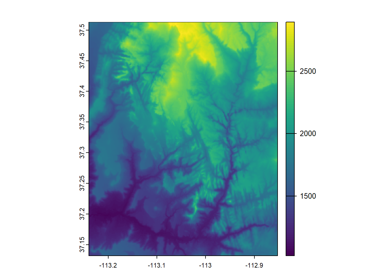
- Advanced Plotting Options:
plotRGB(): A specialized function in terra for creating color composite plots using three layers (e.g., red, green, blue bands) from a SpatRaster object.tmapPackage (Tennekes 2018): Useful for creating both static and interactive maps for raster and vector data.rasterVisPackage (2023): Includes functions such aslevelplot()to create advanced visualizations, including faceted plots for displaying changes over time.
2.3.4 Raster Classes
- The SpatRaster class in
terrarepresents raster objects. Rasters are commonly created by reading a file usingrast()terrasupports reading various formats via GDAL, only loading the header and a file pointer into RAM.
- Creating Rasters from Scratch: Use rast() to make new raster objects:
- Fills values row-wise from the top left corner.
- Resolution depends on rows, columns, and extent; defaults to degrees (WGS84 CRS).
Code
# Create a new SpatRaster object: a checkerboard design
new_raster = rast(nrows = 50, ncols = 50,
                  xmin = 0, xmax = 50,
                  ymin = 0, ymax = 50,
                  vals = rep(c(1, 0.25, 0.75, 0.5),
                             times = 12))


# Plot the new raster
plot(new_raster,
     col = c("darkblue",
             "white",
             "blue",
             "lightblue"), # Use blue and white for the design
     axes = TRUE,
     box = FALSE)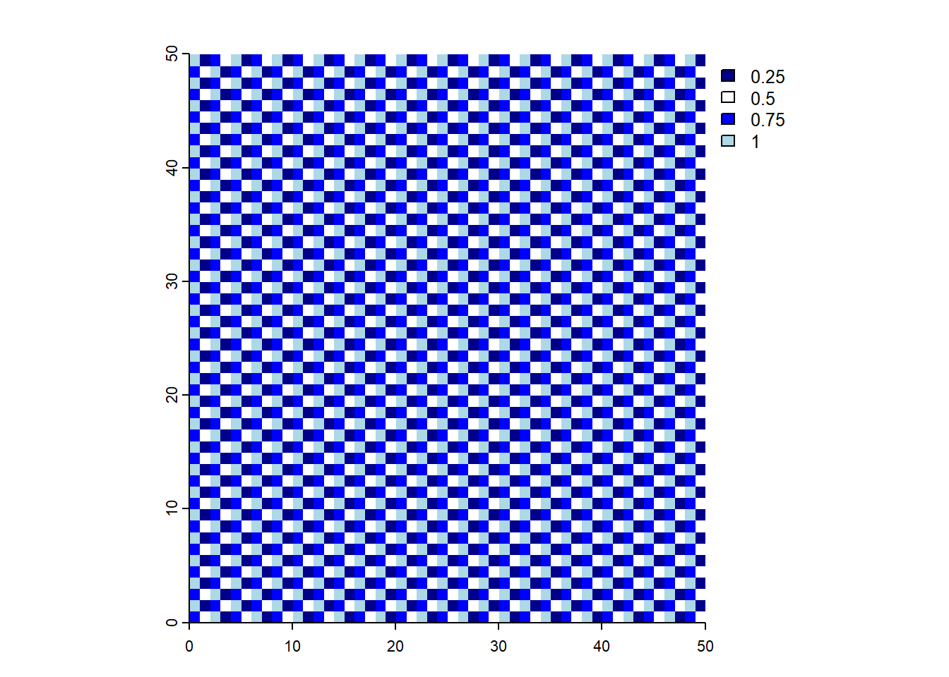
- Handling Multi-Layer Rasters:
SpatRaster supports multi-layer rasters, such as satellite or time-series data:
Use
nlyr()to get the number of layers:Access layers with
[[or$.Use
subset()for layer extraction:
- Combining Raster Layers:
- Merge SpatRaster layers using c():
- Saving SpatRaster Objects:
- Since they often point to files, direct saving to .rds or .rda isn’t feasible.
- Solutions:
wrap(): Creates a temporary object for saving or cluster use.writeRaster(): Saves as a regular raster file.
2.4 Coordinate Reference Systems
- CRSs (Coordinate Reference Systems) are essential for spatial data, defining how spatial elements correspond to the Earth’s surface (or other celestial bodies).
- Types of CRSs:
- Geographic CRSs:
- Represent data on a three-dimensional surface (e.g., latitude and longitude).
- Coordinate units are typically degrees.
- Projected CRSs:
- Represent data on a two-dimensional, flat plane.
- Transform spherical Earth data into a flat map.
- Coordinate units can be in meters, feet, etc.
- Geographic CRSs:
2.4.1 Geographic Coordinate Reference Systems
- Geographic CRSs use longitude and latitude to identify locations on Earth.
- Longitude: Measures East-West position relative to the Prime Meridian.
- Latitude: Measures North-South position relative to the equatorial plane.
- Distances are measured in angular units (degrees), not meters, impacting spatial measurements (explored further in Section 7).
- The Earth can be modeled as spherical or ellipsoidal.
- Spherical models: Simplify calculations by assuming Earth is a perfect sphere.
- Ellipsoidal models: More accurately represent Earth with distinct equatorial and polar radii. The equatorial radius is about 11.5 km longer than the polar radius due to Earth’s compression.
- Datum refers to the model describing the relationship between coordinate values and actual locations on Earth. A datum consists of:
Ellipsoid: An idealized mathematical model of the Earth’s shape, which helps to approximate the Earth’s surface.
Origin Point: A fixed starting point for the coordinate system, where the ellipsoid is anchored to Earth.
Offset and Orientation: How the ellipsoid is aligned with respect to the actual shape of the Earth.
- The two types of Datums are: —
- Geocentric datum (e.g., WGS84): Centered at Earth’s center of gravity, providing global consistency but less local accuracy.
- Local datum (e.g., NAD83): Adjusted for specific regions to better align with the Earth’s surface, accounting for local geographic variations (e.g., mountain ranges).
2.4.2 Projected Coordinate Reference Systems
- Projected CRSs are based on geographic CRSs and use map projections to represent Earth’s three-dimensional surface in Easting and Northing (x and y) values. These CRSs rely on Cartesian coordinates on a flat surface, with an origin and linear units (e.g., meters).
- Deformations:
- The conversion from 3D to 2D inherently introduces distortions. Projected CRSs can only preserve one or two of the following properties:
- Area: Preserved in equal-area projections.
- Direction: Preserved in azimuthal projections.
- Distance: Preserved in equidistant projections.
- Shape: Preserved in conformal projections.
- The conversion from 3D to 2D inherently introduces distortions. Projected CRSs can only preserve one or two of the following properties:
Types of Projections and Their Characteristics
| Type of Projection | Description | Common Properties Preserved | Best Used For |
|---|---|---|---|
| Conic | Projects Earth’s surface onto a cone. | Area, shape | Maps of mid-latitude regions |
| Cylindrical | Projects Earth’s surface onto a cylinder. | Direction, shape | World maps |
| Planar (Azimuthal) | Projects onto a flat surface at a point or line. | Distance, direction | Polar region maps |
Deformations by Projection Type
| Property | Definition | Projection Type That Preserves It |
|---|---|---|
| Area | The relative size of regions is maintained. | Equal-area projections (e.g., Albers) |
| Direction | Bearings from the center are accurate. | Azimuthal projections (e.g., Lambert) |
| Distance | Correct distances are preserved along specific lines or from specific points. | Equidistant projections (e.g., Equirectangular) |
| Shape | Local angles and shapes are maintained, though areas are distorted. | Conformal projections (e.g., Mercator) |
- Use the Map Projection Explorer for details.
- Use
st_crs()for querying CRSs in sf objects andcrs()for terra objects.
Code
sf_proj_info(type = "proj") |>
  as_tibble() |>
  gt::gt() |>
  gt::cols_label_with(fn = snakecase::to_title_case) |>
  gtExtras::gt_theme_espn() |>
gt::opt_interactive()2.5 Units
CRSs include spatial units information, which is crucial for accurately interpreting distance and area.
Cartographic best practices suggest adding scale indicators on maps to show the relationship between map and ground distances.
Units in
sfObjects:sfobjects natively support units for geometric data, ensuring outputs from functions likest_area()come with aunitsattribute.- This feature, supported by the
unitspackage, avoids confusion across different CRSs, which may use meters, feet, etc. - To convert units, use
units::set_units()
Units in Raster Data:
- Unlike
sf, raster packages do not natively support units. - Users should be cautious when working with raster data to convert units properly.
- An example to calculate the area of India in square meters and then, square kilometres
- Unlike
# Load required libraries
library(sf)
library(units)

# Calculate the area of India in square meters
india_area <- rnaturalearth::ne_countries() |>
  filter(admin == "India") |>
  st_area()
india_area
3.150428e+12 [m^2]# Convert area to square kilometers
print(paste("Area of India in square kilometers:", format(set_units(india_area, km^2))))[1] "Area of India in square kilometers: 3150428 [km^2]"# Convert area to hectares
print(paste("Area of India in hectares:", format(set_units(india_area, ha))))[1] "Area of India in hectares: 315042827 [ha]"# Convert area to acres
print(paste("Area of India in acres:", format(set_units(india_area, acre))))[1] "Area of India in acres: 778484666 [acre]"2.6 Exercises
E1
Using summary() on the geometry column of the world data object in the spData package provides valuable information about the spatial characteristics of the dataset:
- Geometry Type:
- The output will indicate the type of geometries present in the
worlddata object. Here, it isMULTIPOLYGONsuggesting that the dataset represents the outlines of countries or regions in MULTIPLOYGON formats.
- The output will indicate the type of geometries present in the
- Number of Countries:
- The summary will show the number of geometries or features present, which corresponds to the number of countries or regions represented in the
worlddataset. Here, it is 177 countries.
- The summary will show the number of geometries or features present, which corresponds to the number of countries or regions represented in the
- Coordinate Reference System (CRS):
- The output will include details about the CRS, and in the present case it is EPSG:4326.
summary((spData::world$geom)) MULTIPOLYGON epsg:4326 +proj=long...
177 0 0 E2
To generate the world map, you can run the following code (as shown in Section 2.2.3):
Code
library(spData)
plot(world[3:6])
plot(world["pop"])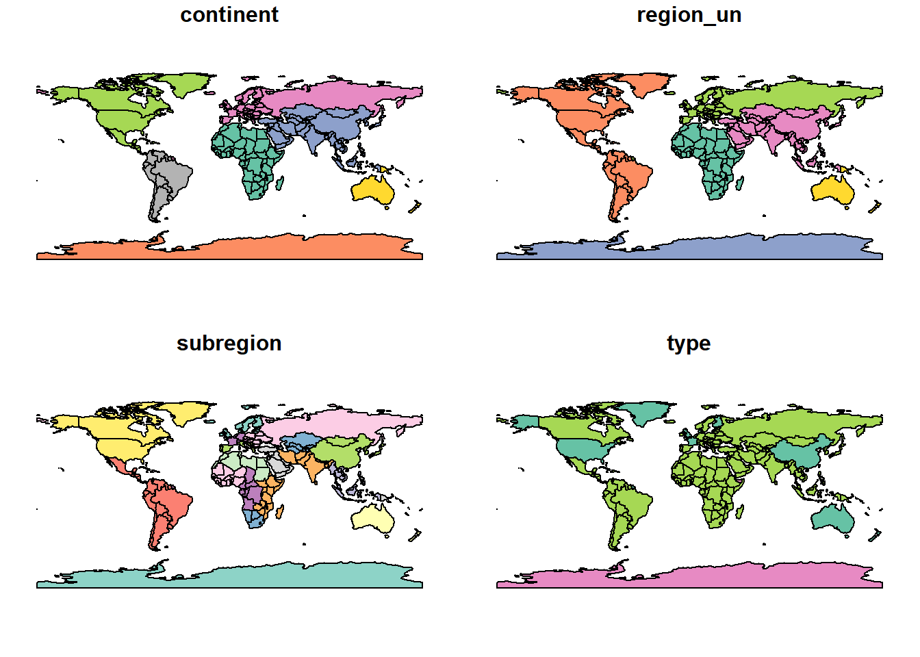
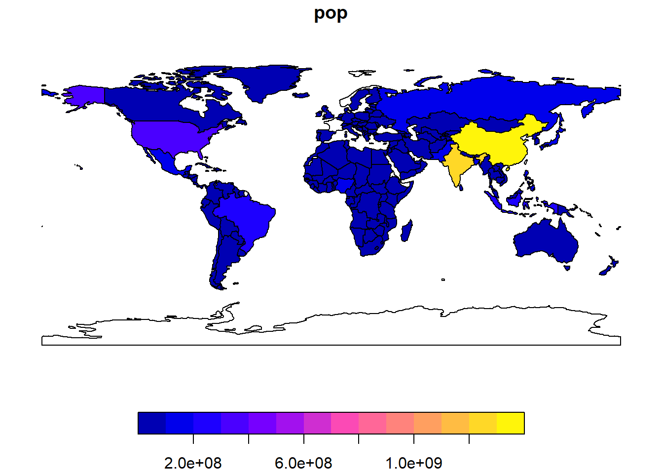
- Similarities:
- The map displays country boundaries and highlights the global population distribution as shown in the book.
- The color scale representing population data is consistent with that described in the book, with larger populations shown with more intense colors.
- Differences:
- The aspect ratio or positioning of the map might vary depending on your screen resolution and window size.
- The color theme and legend display may differ if your R setup or graphic device uses default settings different from those in the book.
cexArgument: This parameter controls the size of plotting symbols in R. It is a numeric value that acts as a multiplier for the default size of symbols.- Setting
cexto values larger than 1 enlarges symbols, while values less than 1 shrink them.
- Setting
- Reason for
cex = sqrt(world$pop) / 10000: The code setscextosqrt(world$pop) / 10000to scale the size of the points on the map in proportion to the population of each country. This square root transformation is used to moderate the variation in symbol sizes because population values can vary significantly between countries. Dividing by 10,000 helps to reduce the symbol size to a reasonable range for plotting.
Other Ideas: —
- Bubble Plot: Overlay a bubble plot on the map with points sized by population.
Code
plot(world["pop"])
points(st_coordinates(st_centroid(world$geom)),
       cex = sqrt(world$pop) / 5000,
       col = "red", pch = 19)
- Choropleth Map: Use color gradients to represent population density.
Code
library(tmap)
tm_shape(world) +
  tm_polygons("pop", style = "jenks",
              palette = "Blues",
              title = "Population")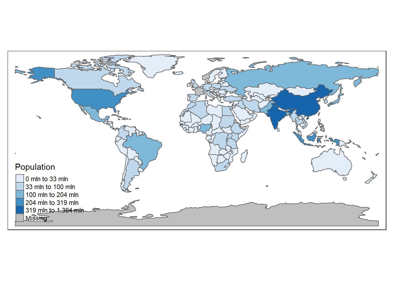
- Log Transformation: Visualize population using a log scale for better differentiation.
Code
world$log_pop = log10(world$pop + 1)
plot(world["log_pop"])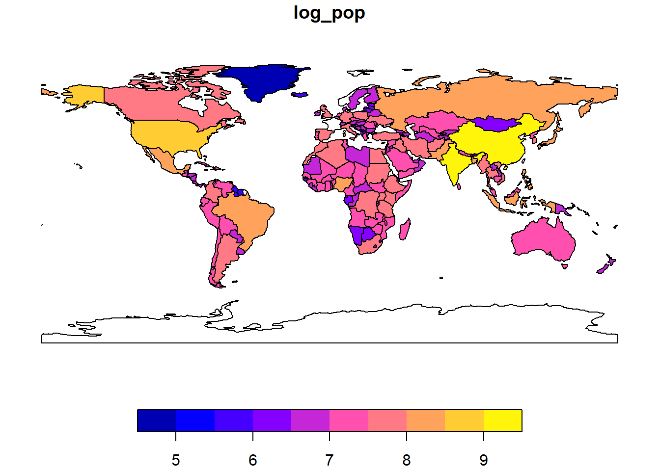
E3
To create a map of Nigeria in context and customize it using the plot() function, you can follow these steps:
Step 1: Load Necessary Libraries and Data: Make sure you have the spData package loaded and access to the world spatial data.
Step 2: Plotting Nigeria in Context: You can plot Nigeria by subsetting the world data and adjusting parameters such as lwd (line width), col (color), and expandBB (expanding the bounding box). Here’s an example code snippet:
Step 3: Annotating the Map: To annotate the map with text labels, you can use the text() function. Here’s an example where we add the name of Nigeria and its capital, Abuja:
Step 4: Exploring the text() Documentation
lwd: This argument controls the line width for the borders of the countries.col: This argument sets the fill color for the countries. You can customize it based on your preference.expandBB: This argument expands the bounding box of the plot, which can help visualize nearby areas more clearly.
E4
To create an empty SpatRaster object with 10 columns and 10 rows, assign random values between 0 and 10, and then plot it, you can use the terra package in R. Here’s how you can do it:
Code
library(terra)

# Create an empty SpatRaster object with 10 columns and 10 rows
my_raster <- rast(nrows = 10, ncols = 10)

# Assign random values between 0 and 10
values(my_raster) <- runif(ncell(my_raster), min = 0, max = 10)

# Plot the raster
plot(my_raster, main = "Random Values Raster")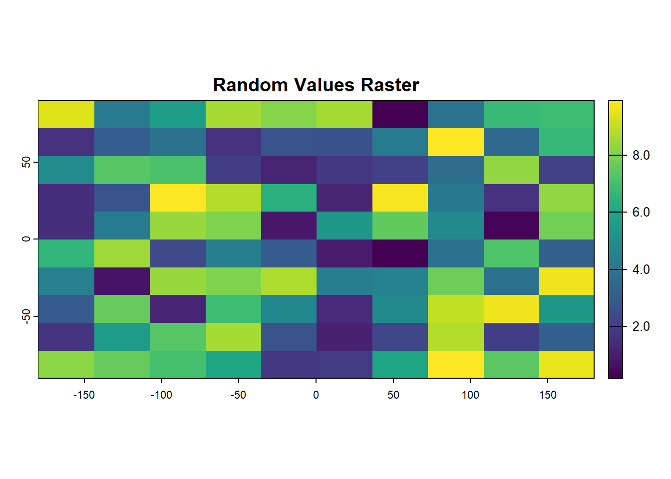
E5
To read in the raster/nlcd.tif file from the spDataLarge package and examine its properties, you can follow these steps in R:
library(spDataLarge)
library(terra)

# Read the raster file
nlcd_raster <- rast(system.file("raster/nlcd.tif", package = "spDataLarge"))
Information You Can Obtain: —
Basic Properties: The
print(nlcd_raster)command will provide you with information about the raster, including its dimensions, number of layers, and type of data.# Check the basic properties of the raster print(nlcd_raster)class : SpatRaster dimensions : 1359, 1073, 1 (nrow, ncol, nlyr) resolution : 31.5303, 31.52466 (x, y) extent : 301903.3, 335735.4, 4111244, 4154086 (xmin, xmax, ymin, ymax) coord. ref. : NAD83 / UTM zone 12N (EPSG:26912) source : nlcd.tif color table : 1 categories : levels name : levels min value : Water max value : WetlandsSummary Statistics: The
summary(nlcd_raster)function will give you basic statistics about the raster values, such as minimum, maximum, and mean values. In this case, it tells the number of cells with Forest, Shrubland, Barren, Developed, Cultivated, Wetlands and Other land-use types.# Get summary statistics summary(nlcd_raster)levels Forest :52620 Shrubland :37463 Barren : 7290 Developed : 1203 Cultivated: 596 Wetlands : 443 (Other) : 421Extent: The
ext(nlcd_raster)command will provide the geographical extent of the raster, showing the minimum and maximum x and y coordinates.# Check the extent of the raster ext(nlcd_raster)SpatExtent : 301903.344386758, 335735.354381954, 4111244.46098842, 4154086.47216415 (xmin, xmax, ymin, ymax)Rows and Columns: You can find the number of rows and columns in the raster using
nrow(nlcd_raster)andncol(nlcd_raster).# Get the number of rows and columns nrow(nlcd_raster)[1] 1359ncol(nlcd_raster)[1] 1073Coordinate Reference System (CRS): The
crs(nlcd_raster)command will return the CRS of the raster, which is essential for spatial analyses.# Get the coordinate reference system (CRS) str_view(crs(nlcd_raster))[1] │ PROJCRS["NAD83 / UTM zone 12N", │ BASEGEOGCRS["NAD83", │ DATUM["North American Datum 1983", │ ELLIPSOID["GRS 1980",6378137,298.257222101, │ LENGTHUNIT["metre",1]]], │ PRIMEM["Greenwich",0, │ ANGLEUNIT["degree",0.0174532925199433]], │ ID["EPSG",4269]], │ CONVERSION["UTM zone 12N", │ METHOD["Transverse Mercator", │ ID["EPSG",9807]], │ PARAMETER["Latitude of natural origin",0, │ ANGLEUNIT["degree",0.0174532925199433], │ ID["EPSG",8801]], │ PARAMETER["Longitude of natural origin",-111, │ ANGLEUNIT["degree",0.0174532925199433], │ ID["EPSG",8802]], │ PARAMETER["Scale factor at natural origin",0.9996, │ SCALEUNIT["unity",1], │ ID["EPSG",8805]], │ PARAMETER["False easting",500000, │ LENGTHUNIT["metre",1], │ ID["EPSG",8806]], │ PARAMETER["False northing",0, │ LENGTHUNIT["metre",1], │ ID["EPSG",8807]]], │ CS[Cartesian,2], │ AXIS["(E)",east, │ ORDER[1], │ LENGTHUNIT["metre",1]], │ AXIS["(N)",north, │ ORDER[2], │ LENGTHUNIT["metre",1]], │ USAGE[ │ SCOPE["Engineering survey, topographic mapping."], │ AREA["North America - between 114°W and 108°W - onshore and offshore. Canada - Alberta; Northwest Territories; Nunavut; Saskatchewan. United States (USA) - Arizona; Colorado; Idaho; Montana; New Mexico; Utah; Wyoming."], │ BBOX[31.33,-114,84,-108]], │ ID["EPSG",26912]]Resolution: You can check the resolution of the raster with the
res(nlcd_raster)function, which will indicate the size of each pixel.# Check the resolution of the raster res(nlcd_raster)[1] 31.53030 31.52466Values: The
values(nlcd_raster)command allows you to access the actual values contained in the raster. Here, I am printing only the first few values.# Get the values of the raster values(nlcd_raster) |> head()levels [1,] 4 [2,] 4 [3,] 5 [4,] 4 [5,] 4 [6,] 4
E6
To check the Coordinate Reference System (CRS) of the raster/nlcd.tif file from the spDataLarge package, you can use the following steps in R. The CRS provides essential information about how the spatial data is projected on the Earth’s surface.
library(spDataLarge)
library(terra)

# Read the raster file
nlcd_raster <- rast(system.file("raster/nlcd.tif", package = "spDataLarge"))

# Check the coordinate reference system (CRS)
nlcd_crs <- crs(nlcd_raster)
nlcd_crs |> str_view()
[1] │ PROJCRS["NAD83 / UTM zone 12N",
│ BASEGEOGCRS["NAD83",
│ DATUM["North American Datum 1983",
│ ELLIPSOID["GRS 1980",6378137,298.257222101,
│ LENGTHUNIT["metre",1]]],
│ PRIMEM["Greenwich",0,
│ ANGLEUNIT["degree",0.0174532925199433]],
│ ID["EPSG",4269]],
│ CONVERSION["UTM zone 12N",
│ METHOD["Transverse Mercator",
│ ID["EPSG",9807]],
│ PARAMETER["Latitude of natural origin",0,
│ ANGLEUNIT["degree",0.0174532925199433],
│ ID["EPSG",8801]],
│ PARAMETER["Longitude of natural origin",-111,
│ ANGLEUNIT["degree",0.0174532925199433],
│ ID["EPSG",8802]],
│ PARAMETER["Scale factor at natural origin",0.9996,
│ SCALEUNIT["unity",1],
│ ID["EPSG",8805]],
│ PARAMETER["False easting",500000,
│ LENGTHUNIT["metre",1],
│ ID["EPSG",8806]],
│ PARAMETER["False northing",0,
│ LENGTHUNIT["metre",1],
│ ID["EPSG",8807]]],
│ CS[Cartesian,2],
│ AXIS["(E)",east,
│ ORDER[1],
│ LENGTHUNIT["metre",1]],
│ AXIS["(N)",north,
│ ORDER[2],
│ LENGTHUNIT["metre",1]],
│ USAGE[
│ SCOPE["Engineering survey, topographic mapping."],
│ AREA["North America - between 114°W and 108°W - onshore and offshore. Canada - Alberta; Northwest Territories; Nunavut; Saskatchewan. United States (USA) - Arizona; Colorado; Idaho; Montana; New Mexico; Utah; Wyoming."],
│ BBOX[31.33,-114,84,-108]],
│ ID["EPSG",26912]]Understanding the CRS Information: —
The output from the crs(nlcd_raster) command will typically include details such as:
Projection Type: Indicates whether the CRS is geographic (latitude and longitude) or projected (a flat representation). Here, it is North American NAD83 / UTM Zone 12 N
Datum: Information about the geodetic datum used, which is crucial for accurately locating points on the Earth’s surface. Here, it is North American Datum 1983.
Coordinate Units: Specifies the units of measurement used for the coordinates, such as degrees (for geographic CRSs) or meters (for projected CRSs). Here, it is in metres, as shown in:
LENGTHUNIT["metre",1]EPSG Code: If applicable, the output might include an EPSG code, which is a standardized reference number for a specific CRS. This code can be used to look up more detailed information about the CRS. Here, it is: —
ID["EPSG",26912]Transformation Parameters: If it’s a projected CRS, the output may include parameters related to the projection method, such as central meridian, standard parallels, and false easting/northing. Here, they are: —
|         PRIMEM["Greenwich",0,
│             ANGLEUNIT["degree",0.0174532925199433]],
│         ID["EPSG",4269]],
|
|
│     CONVERSION["UTM zone 12N",
│         METHOD["Transverse Mercator",
│             ID["EPSG",9807]],
│         PARAMETER["Latitude of natural origin",0,
│             ANGLEUNIT["degree",0.0174532925199433],
│             ID["EPSG",8801]],
│         PARAMETER["Longitude of natural origin",-111,
|             ANGLEUNIT["degree",0.0174532925199433],
│             ID["EPSG",8802]],
│         PARAMETER["Scale factor at natural origin",0.9996,
│             SCALEUNIT["unity",1],
│             ID["EPSG",8805]],
│         PARAMETER["False easting",500000,
│             LENGTHUNIT["metre",1],
│             ID["EPSG",8806]],
│         PARAMETER["False northing",0,
│             LENGTHUNIT["metre",1],
│             ID["EPSG",8807]]],
References
Cooley, David. 2024. “Sfheaders: Converts Between r Objects and Simple Feature Objects.” https://CRAN.R-project.org/package=sfheaders.
Oscar Perpiñán, and Robert Hijmans. 2023. “rasterVis.” https://oscarperpinan.github.io/rastervis/.
Tennekes, Martijn. 2018. “Tmap: Thematic Maps in r” 84. https://doi.org/10.18637/jss.v084.i06.