library(sf)        # Simple Features in R
library(terra)     # Handling rasters in R
library(tidyterra) # For plotting rasters in ggplot2
library(magrittr)  # Using pipes with raster objects
library(tidyverse) # All things tidy; Data Wrangling
library(spData)    # Spatial Datasets


sysfonts::font_add_google("Saira Extra Condensed", "caption_font")
sysfonts::font_add_google("Saira", "body_font")
theme_set(theme_minimal(base_family = "body_font",
                        base_size = 16))
showtext::showtext_auto()Chapter 4: Spatial data operations
Key Learnings from, and Solutions to the exercises in Chapter 4 of the book Geocomputation with R by Robin Lovelace, Jakub Nowosad and Jannes Muenchow.
4.1 Introduction to Spatial Operations
- Spatial Operations: Include spatial joins for vectors and local/focal operations for rasters, allowing modification based on location and shape.
- Relation to Non-Spatial Operations: Many spatial operations (e.g., subsetting, joining) have non-spatial counterparts.
- Spatial Joins: Can be done in multiple ways (e.g., intersect, within distance), unlike non-spatial joins (refer to fuzzyjoin package (Robinson 2020) for alternatives).
- Types of Spatial Relationships: Includes operations like intersects and disjoint. Distance calculations explore spatial relationships.
- Raster Operations:
- Subsetting (Section 4.3.1)
- Map Algebra: Modifies raster cell values through local, focal, zonal, and global operations (Sections 4.3.3 to 4.3.6).
- Merging Rasters: Demonstrated with reproducible examples (Section 4.3.8).
- Coordinate Reference System (CRS): Consistency in CRS is essential for spatial operations..
4.2 Spatial operations on vector data
4.2.1 Spatial Subsetting: use st_filter()
- Spatial subsetting extracts features from a spatial object (
x) that relate spatially to another object (y). - Syntax: Use the
[ ]operator:x[y, , op = st_intersects].x: Targetsfobject.y: Subsettingsfobject.op: Topological relation (default isst_intersects).
- Default Operator:
st_intersects()selects features intersecting with the subsetting object. Alternative operators likest_disjoint()can be used for different relations.- Example:
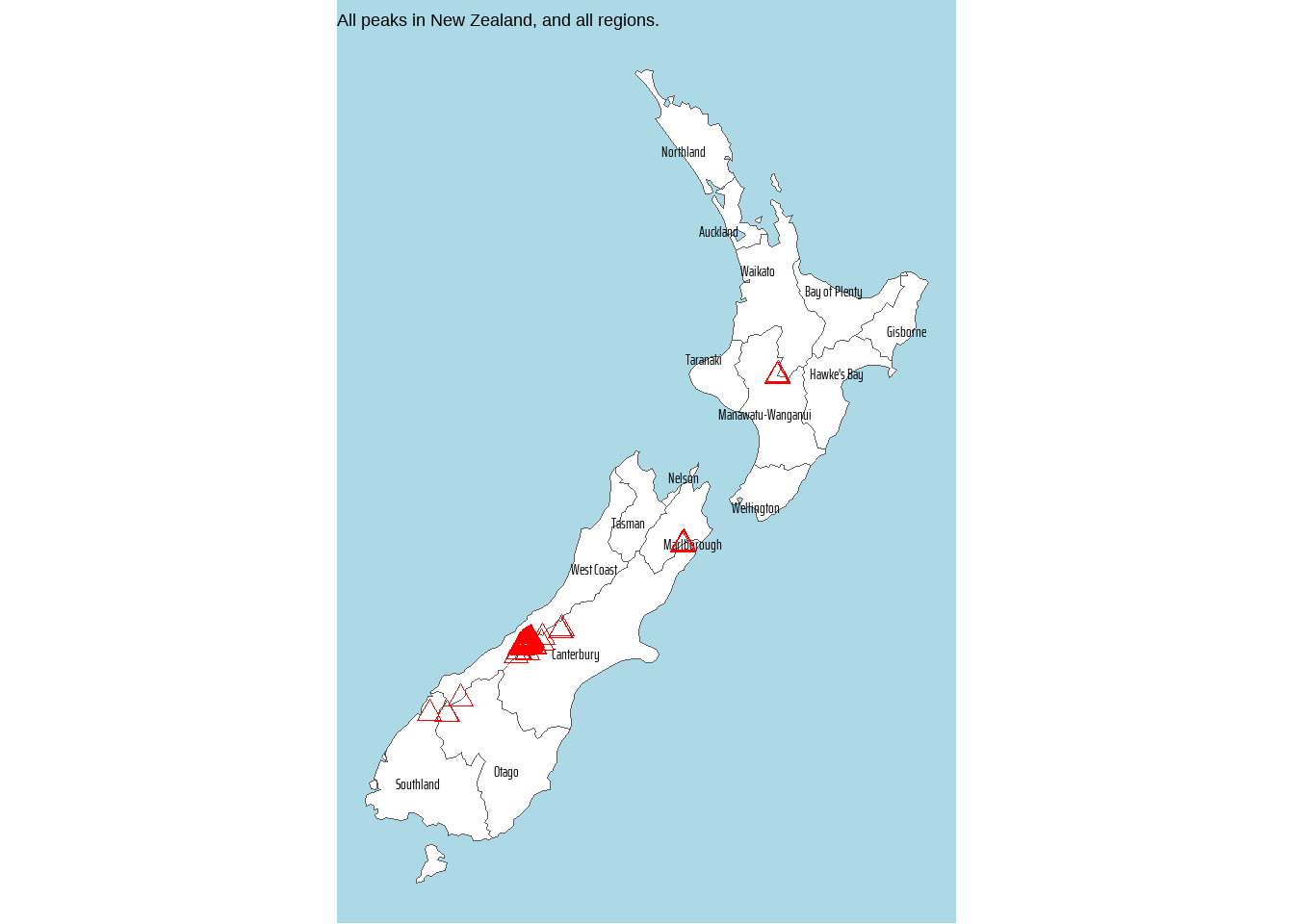
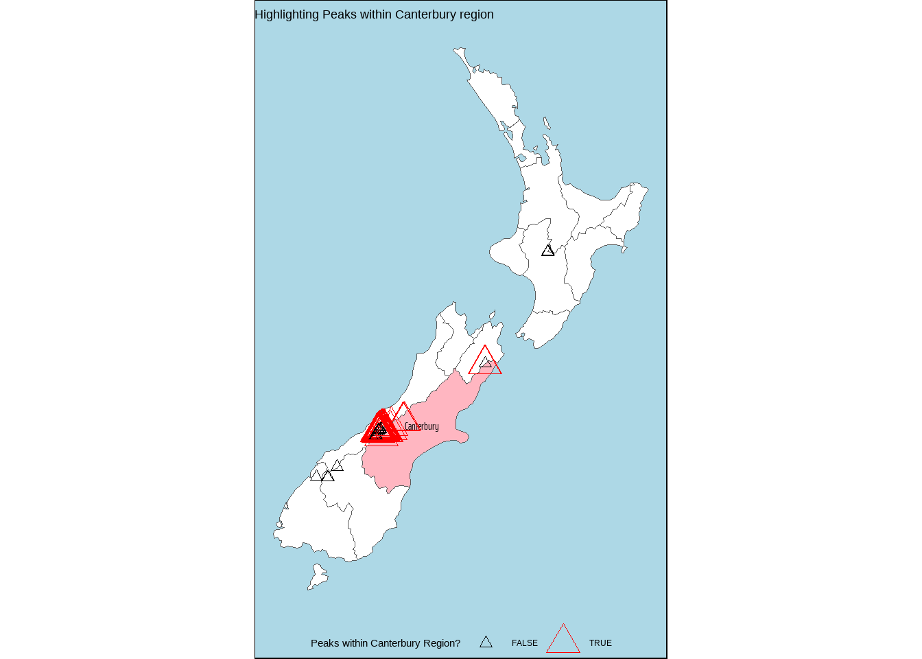
nz_height[canterbury, ]returns high points within Canterbury from thenz_heightdataset in the spData package (spData documentation).
- Example:
- Topological Relations: Include
touches,crosses, andwithin. These determine spatial relationships between features inxandy. - Sparse Geometry Binary Predicate (sgbp):
- Using
st_intersects(), ansgbplist object is created. - Convert
sgbpto logical vector for subsetting usinglengths({sgbp_object_name} > 0) - Using
sparse = FALSEargument inst_intersects()returns a dense matrix.
- Using
- Tidyverse Alternative:
st_filter()from the sf package simplifies spatial subsetting, increasing compatibility withdplyr. - Output Consistency: Subsets created using
[ ], logical vectors, orst_filter()are equivalent in spatial operations.
Code
data("nz")
data("nz_height")

class(nz)
## [1] "sf"         "data.frame"

# A plot for all regions and all peaks
nz |>
  ggplot() +
  geom_sf(fill = "white") +
  ggrepel::geom_text_repel(
    mapping = aes(
      label = Name,
      geometry = geom
    ),
    size = 4,
    family = "caption_font",
    stat = "sf_coordinates"
  ) +
  geom_sf(
    data = nz_height,
    pch = 2,
    colour = "red",
    size = 3
  ) +
  scale_fill_manual(
    values = c("white", "pink")
  ) +
  labs(
    title = "All peaks in New Zealand, and all regions."
  ) +
  theme_void() +
  theme(
    plot.background = element_rect(
      fill = "lightblue",
      colour = NA
    ),
    legend.position = "none"
  )

# Total peaks in New Zealand
nz_height |> dim()
## [1] 101   3

# Peaks within Canterbury in New Zealand

# Base R Version
canterbury <- nz |> filter(Name == "Canterbury")
nz_height[canterbury,] |> dim()
## [1] 70  3

# Tidyverse Version
nz_height |>
  st_filter(
    nz |> filter(Name == "Canterbury"),
    .predicate = st_intersects
  ) |>
  dim()
## [1] 70  3

# Getting the peaks which are inside Canterbury
canterbury_ids <- nz_height |>
  st_filter(
    nz |> filter(Name == "Canterbury"),
    .predicate = st_intersects
  ) |>
  pull(t50_fid)

nz_height |>
  mutate(in_canterbury = t50_fid %in% canterbury_ids) |>
  ggplot() +

  # Base NZ Map and Label for Canterbury
  geom_sf(
    data = nz,
    mapping = aes(
      fill = Name == "Canterbury"
    )
  ) +
  geom_sf_text(
    data = filter(nz, Name == "Canterbury"),
    mapping = aes(
      label = Name,
      geometry = geom
    ),
    size = 4,
    family = "caption_font"
  ) +

  # Plotting the peaks, and colouring by presence in Canterbury
  geom_sf(
    mapping = aes(
      colour = in_canterbury,
      size = in_canterbury
    ),
    pch = 2
  ) +

  scale_fill_manual(
    values = c("white", "lightpink")
  ) +
  scale_colour_manual(
    values = c("black", "red")
  ) +
  guides(
    fill = "none"
  ) +
  labs(
    colour = "Peaks within Canterbury Region?",
    size = "Peaks within Canterbury Region?",
    title = "Highlighting Peaks within Canterbury region"
  ) +
  theme_void() +
  theme(
    plot.background = element_rect(
      fill = "lightblue"
    ),
    legend.position = "bottom"
)Example code for st_intersects() and st_disjoint() : these functions produce a sparse predicate list only. Hence, correct way to use them would be st_filter() with .predicate = <function> argument.
nz_height |>
  st_intersects(
    filter(nz, Name == "Canterbury")
  )
Sparse geometry binary predicate list of length 101, where the
predicate was `intersects'
first 10 elements:
1: (empty)
2: (empty)
3: (empty)
4: (empty)
5: 1
6: 1
7: 1
8: 1
9: 1
10: 1# The 70 peaks within Canterbury region
nz_height |>
st_filter(
filter(nz, Name == "Canterbury"),
.predicate = st_intersects
)Simple feature collection with 70 features and 2 fields
Geometry type: POINT
Dimension: XY
Bounding box: xmin: 1365809 ymin: 5158491 xmax: 1654899 ymax: 5350463
Projected CRS: NZGD2000 / New Zealand Transverse Mercator 2000
First 10 features:
t50_fid elevation geometry
1 2362630 2749 POINT (1378170 5158491)
2 2362814 2822 POINT (1389460 5168749)
3 2362817 2778 POINT (1390166 5169466)
4 2363991 3004 POINT (1372357 5172729)
5 2363993 3114 POINT (1372062 5173236)
6 2363994 2882 POINT (1372810 5173419)
7 2363995 2796 POINT (1372579 5173989)
8 2363997 3070 POINT (1373796 5174144)
9 2363998 3061 POINT (1373955 5174231)
10 2363999 3077 POINT (1373984 5175228)# The 31 peaks outside Canterbury Region
nz_height |>
st_filter(
filter(nz, Name == "Canterbury"),
.predicate = st_disjoint
)Simple feature collection with 31 features and 2 fields
Geometry type: POINT
Dimension: XY
Bounding box: xmin: 1204143 ymin: 5048309 xmax: 1822492 ymax: 5650492
Projected CRS: NZGD2000 / New Zealand Transverse Mercator 2000
First 10 features:
t50_fid elevation geometry
1 2353944 2723 POINT (1204143 5049971)
2 2354404 2820 POINT (1234725 5048309)
3 2354405 2830 POINT (1235915 5048745)
4 2369113 3033 POINT (1259702 5076570)
5 2363996 2759 POINT (1373264 5175442)
6 2364028 2756 POINT (1374183 5177165)
7 2364029 2800 POINT (1374469 5176966)
8 2364031 2788 POINT (1375422 5177253)
9 2364166 2782 POINT (1383006 5181085)
10 2364167 2905 POINT (1383486 5181270)4.2.2 Topological Relations
- Topological relations describe spatial relationships between objects using logical TRUE or FALSE statements (Egenhofer and Herring, 1990).
- Symmetrical vs. non-symmetrical relations:
- Symmetrical relations (e.g.,
equals,intersects,crosses) yield the same result when order of input is swapped. - Non-symmetrical relations (e.g.,
contains,within) depend on the order of input geometries.
- Symmetrical relations (e.g.,
- Binary predicates in
sfpackage test spatial relationships between vector geometries. See vignette(“sf3”). The following binary predicates exist insf: —
| Function | Description | Symmetrical? |
|---|---|---|
st_intersects |
Checks if geometries intersect. | Yes |
st_disjoint |
Checks if geometries do not intersect (are disjoint). | Yes |
st_touches |
Checks if geometries have at least one boundary point in common. | Yes |
st_crosses |
Checks if a geometry crosses another (e.g., a line crosses a polygon). | Yes |
st_overlaps |
Checks if geometries have some but not all interior points in common. | Yes |
st_equals |
Checks if geometries are topologically equal. | Yes |
st_within |
Checks if a geometry is completely contained within another. | No |
st_contains |
Checks if a geometry contains another completely. | No |
st_contains_properly |
Checks if a geometry contains another but not vice versa. | No |
st_covers |
Checks if a geometry covers another (includes boundary). | No |
st_covered_by |
Checks if a geometry is covered by another (includes boundary). | No |
st_equals_exact |
Checks if geometries are exactly equal within a given tolerance. | Yes |
st_is_within_distance |
Checks if geometries are within a specified distance from each other. | Yes |
- Sparse matrix output: Functions like
st_intersects()use sparse matrices to save memory by only registering positive results; settingsparse = FALSEreturns a dense matrix.
Code
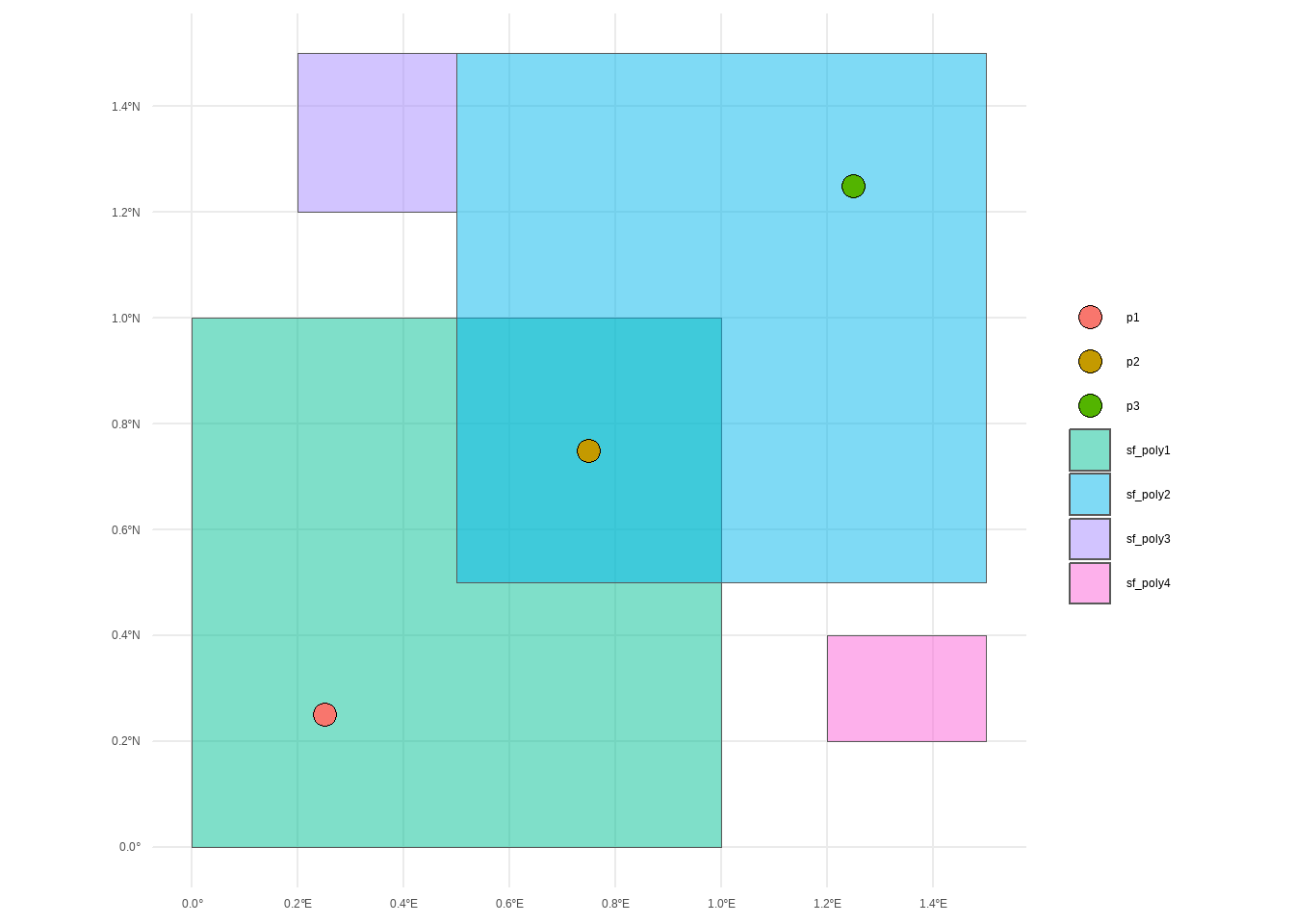
# Create two polygons
 polygon1 <- st_polygon(
   list(matrix(c(0, 0, 1, 0, 1, 1, 0, 1, 0, 0),
     ncol = 2,
     byrow = TRUE
   ))
 )

 polygon2 <- st_polygon(
   list(matrix(c(0.5, 0.5, 1.5, 0.5, 1.5, 1.5, 0.5, 1.5, 0.5, 0.5),
     ncol = 2,
     byrow = TRUE
   ))
 )

 polygon3 <- st_polygon(
   list(matrix(c(0.2, 1.2,
                 0.5, 1.2,
                 0.5, 1.5,
                 0.2, 1.5,
                 0.2, 1.2),
     ncol = 2,
     byrow = TRUE
   ))
 )

 polygon4 <- st_polygon(
   list(matrix(c(1.2, 0.2,
                 1.5, 0.2,
                 1.5, 0.4,
                 1.2, 0.4,
                 1.2, 0.2),
     ncol = 2,
     byrow = TRUE
   ))
 )

 # Convert to sf objects
 sf_poly1 <- st_sfc(polygon1, crs = 4326)
 sf_poly2 <- st_sfc(polygon2, crs = 4326)
 sf_poly3 <- st_sfc(polygon3, crs = 4326)
 sf_poly4 <- st_sfc(polygon4, crs = 4326)

 # Create a collection of points
 points <- st_sfc(
   st_point(c(0.25, 0.25)),
   st_point(c(0.75, 0.75)),
   st_point(c(1.25, 1.25)),
   crs = 4326
 )

 sf_points <- tibble(
   point = c("p1", "p2", "p3"),
   geometry = points
 ) |>
   st_as_sf() |>
   st_set_crs(4326)

# Keeping environment clean
rm(polygon1, polygon2,
   polygon3, polygon4,
   points)

# Visualize the objects
ggplot() +
  geom_sf(data = sf_poly1,
          aes(fill = "sf_poly1"),
          alpha = 0.5) +
  geom_sf(data = sf_poly2,
          aes(fill = "sf_poly2"),
          alpha = 0.5) +
  geom_sf(data = sf_poly3,
          aes(fill = "sf_poly3"),
          alpha = 0.5) +
  geom_sf(data = sf_poly4,
          aes(fill = "sf_poly4"),
          alpha = 0.5) +
  geom_sf(data = sf_points,
          aes(fill = point),
          pch = 21,
          size = 4) +
  labs(fill = NULL) +
theme_minimal()#################### Symmetrical Relations ######################
# The order in which sf objects are placed does not matter
## st_intersects()----------------------------------------
st_intersects(sf_poly1, sf_poly2, sparse = F)
## [,1]
## [1,] TRUE
st_intersects(sf_poly1, sf_points, sparse = F)
## [,1] [,2] [,3]
## [1,] TRUE TRUE FALSE
st_intersects(sf_poly1, sf_poly3, sparse = F)
## [,1]
## [1,] FALSE
st_intersects(sf_poly2 ,sf_poly3, sparse = F)
## [,1]
## [1,] TRUE
# st_disjoint()------------------------------------------
st_disjoint(sf_poly1, sf_poly4, sparse = F)
## [,1]
## [1,] TRUE
st_disjoint(sf_poly2, sf_poly3, sparse = F)
## [,1]
## [1,] FALSE
# st_touches()-------------------------------------------
st_touches(sf_poly1, sf_poly2, sparse = F)
## [,1]
## [1,] FALSE
st_touches(sf_poly2, sf_poly3, sparse = F)
## [,1]
## [1,] TRUE
st_touches(sf_poly1, sf_points, sparse = F)
## [,1] [,2] [,3]
## [1,] FALSE FALSE FALSE
# st_crosses()-------------------------------------------
st_crosses(sf_poly1, sf_poly2, sparse = F)
## [,1]
## [1,] FALSE
st_crosses(sf_poly1, sf_points, sparse = F)
## [,1] [,2] [,3]
## [1,] FALSE FALSE FALSE
# st_overlaps()
st_overlaps(sf_poly1, sf_poly2, sparse = F)
## [,1]
## [1,] TRUE
st_overlaps(sf_poly1, sf_points, sparse = F)
## [,1] [,2] [,3]
## [1,] FALSE FALSE FALSE
st_overlaps(sf_poly3, sf_poly3, sparse = F)
## [,1]
## [1,] FALSE
# st_equals()-------------------------------------------
st_equals(sf_poly1, sf_poly1, sparse = F)
## [,1]
## [1,] TRUE
# st_equals_exact()-------------------------------------
st_equals_exact(sf_poly1, sf_poly2, par = 0.1, sparse = F)
## [,1]
## [1,] FALSE
st_equals_exact(sf_poly1, sf_poly2, par = 1, sparse = F)
## [,1]
## [1,] TRUE
# st_is_within_distance()-------------------------------
st_is_within_distance(sf_poly1, sf_poly2, dist = 0.1, sparse = F)
## [,1]
## [1,] TRUE
st_is_within_distance(sf_poly2, sf_poly3, dist = 0.1, sparse = F)
## [,1]
## [1,] TRUE
st_is_within_distance(sf_poly3, sf_poly4, dist = 0.1, sparse = F)
## [,1]
## [1,] FALSE
st_is_within_distance(sf_poly3, sf_poly4, dist = 13, sparse = F)
## [,1]
## [1,] FALSE
#################### Non-Symmetrical Relations ####################
# The order in which sf objects are placed changes the outcome
# st_within()-------------------------------------------
sf_points |>
st_within(sf_poly1, sparse = F)
## [,1]
## [1,] TRUE
## [2,] TRUE
## [3,] FALSE
sf_poly1 |>
st_within(sf_points, sparse = F)
## [,1] [,2] [,3]
## [1,] FALSE FALSE FALSE
sf_poly1 |>
st_within(sf_poly2, sparse = F)
## [,1]
## [1,] FALSE
# st_contains()-----------------------------------------
sf_poly1 |>
st_contains(sf_points, sparse = F)
## [,1] [,2] [,3]
## [1,] TRUE TRUE FALSE
sf_points |>
st_contains(sf_poly1, sparse = F)
## [,1]
## [1,] FALSE
## [2,] FALSE
## [3,] FALSE
# st_covers()-------------------------------------------
sf_poly1 |>
st_covers(sf_points, sparse = F)
## [,1] [,2] [,3]
## [1,] TRUE TRUE FALSE
sf_poly2 |>
st_covers(sf_poly1, sparse = F)
## [,1]
## [1,] FALSE
# st_covered_by()---------------------------------------
sf_points |>
st_covered_by(sf_poly1, sparse = F)
## [,1]
## [1,] TRUE
## [2,] TRUE
## [3,] FALSE4.2.3 Distance Relations
- Distance relations are continuous, unlike binary topological relations which return TRUE/FALSE values.
- The
st_distance()function calculates distances between two sf objects, returning a matrix with units of measurement (e.g., meters). st_centroid(): Computes the geometric centroid of a spatial feature, useful for representing a region’s central point in distance calculations.- Matrix output:
- Results are returned as a matrix, even for single value calculations.
- Computes a distance matrix between all combinations of features in objects (e.g., distances between multiple points and polygons).
- Point-to-polygon distance: Represents the shortest distance from a point to any part of the polygon.
- Usage in distance-based joins:
st_distance()is also used for performing joins based on distance criteria. - An example code to find distance between central points of Auckland and Canterbury Regions, vs. Top three peaks in New Zealand, returned as a matrix,a nd shown below as a beautiful table using {gt}.
# Central points of Auckland and Canterbury Regions
df1 <- nz |>
  filter(str_detect(Name, "Auck|Canter")) |>
  st_centroid() |>
  select(Name, geom)

# Top 3 highest peaks in New Zealand
df2 <- nz_height |>
  slice_max(order_by = elevation, n = 3)

# Finding the distance matrix
st_distance(df1, df2) |>
  as_tibble() |>
  mutate(state = c("Auckland", "Canterbury")) |>
  relocate(state) |>
  mutate(
    across(
      .cols = -state,
      .fns = as.numeric
    )
  ) |>
  gt::gt() |>
  gt::fmt_number(
    decimals = 1,
    scale_by = 1e-3
  ) |>
  gt::cols_label(V1 = "Highest Peak",
                 V2 = "Second",
                 V3 = "Third",
                 state = "Centroid of the State") |>
  gt::tab_header(
    title = "Distance in kilometers"
  ) |>
gtExtras::gt_theme_538()| Distance in kilometers | |||
|---|---|---|---|
| Centroid of the State | Highest Peak | Second | Third |
| Auckland | 856.6 | 857.3 | 856.9 |
| Canterbury | 115.5 | 115.4 | 115.5 |
4.2.4 DE-9IM Strings
- The Dimensionally Extended 9-Intersection Model (DE-9IM) underlies binary spatial predicates. This model forms the basis for many spatial operations and helps create custom spatial predicates.
- Origins:
- Initially named “DE + 9IM,” it refers to the dimensions of intersections between the boundaries, interiors, and exteriors of two geometries (Clementini and Di Felice 1995).
- It applies to two-dimensional geometries (points, lines, polygons) in Euclidean space, requiring data in a projected coordinate reference system (CRS).
- How DE-9IM Works:
- The model visualizes intersections between components of two geometries (interior, boundary, exterior) in a 3x3 matrix form, indicating the dimension of the intersection (0 for points, 1 for lines, 2 for polygons, and F for false).
- Flattening this matrix row-wise results in the DE-9IM string: “212111212”.
- Using
st_relate(): Thest_relate()function returns DE-9IM strings to describe spatial relations. - Developing Custom Predicates:
- By interpreting DE-9IM strings, custom binary spatial predicates like queen and rook relations can be created:
Queen relations (shared border or point): Pattern
F***T****.Rook relations (shared linear intersection): Pattern
F***1****.
- Custom functions using
st_relate():
- By interpreting DE-9IM strings, custom binary spatial predicates like queen and rook relations can be created:
st_queen = function(x, y)
  st_relate(x, y, pattern = "F***T****")

st_rook = function(x, y)
st_relate(x, y, pattern = "F***1****")- This identifies which geometries in a grid have queen or rook relations to the central geometry.
4.2.5 Spatial Joining with st_join()
Spatial joins combine datasets based on spatial relationships instead of shared key variables (as in non-spatial joins). It adds columns from a source object (
y) to a target object (x).Join Details:
Default behavior: A left join, which retains all rows from
xand includes rows with no match fromy.Operators: Uses
st_intersects()by default but can be modified via thejoinargument.Handles all geometry types: Works for points, lines, and polygons, though joins involving polygons may create duplicate rows for multiple matches in
y.
Flexibility:
- Inner joins: Set
left = FALSEto include only matched rows.
- Inner joins: Set
The
st_join()function: Thejoinargument defines the topological operator to determine these relationships, with the default beingst_intersects().We can customize this behavior by choosing alternative functions such as
st_contains,st_within,st_overlaps,st_touches, orst_disjoint, among others, each defining a different geometric predicate.For example,
st_containsselects features where geometries ofxfully encompass those ofy, whilest_withindoes the reverse.Additionally, advanced options like
st_is_within_distanceallow proximity-based joins, andst_relatesupports customized spatial relationships using a pattern.
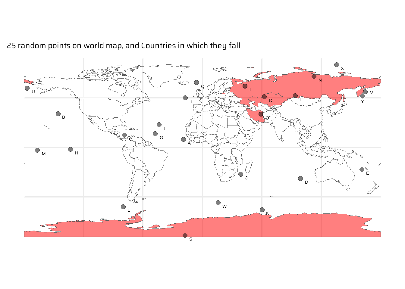
Example: Getting 25 random points in the world, and seeing in which countries they fall in Figure 3.
Code
# Getting 25 random points on the world,a dn then seeing in which countries they fall
random_points <- tibble(
  x = round(
    runif(
    25,
    min = st_bbox(world)$xmin,
    max = st_bbox(world)$xmax
    ),
    2
  ),
  y = round(
    runif(
    25,
    min = st_bbox(world)$ymin,
    max = st_bbox(world)$ymax
    ),
    2
  ),
  id = LETTERS[1:25]
) |>
  st_as_sf(coords = c("x", "y")) |>
  st_set_crs(value = crs(world))


# Easiest (but not tidyverse) way to subset
# world[random_points, ]

# Tidyverse way to filter: Names of Countries in which they fall
intersecting_countries <- world |>
  st_filter(random_points) |>
  pull(name_long)

# The power of spatial joins: A tibble of countries where each random
# point falls. st_join() by default performs a left_join()
st_join(
  random_points,
  world |> select(name_long)
) |>
  drop_na() |>
  gt::gt() |>
gtExtras::gt_theme_nytimes()| id | geometry | name_long |
|---|---|---|
| I | c(43.05, 61.96) | Russian Federation |
| N | c(112.59, 71.68) | Russian Federation |
| O | c(59.22, 33.55) | Iran |
| P | c(93.88, 52.24) | Russian Federation |
| R | c(62.63, 51.25) | Kazakhstan |
| S | c(-17.61, -88.84) | Antarctica |
Code
set.seed(42)

world |>
  mutate(highlight = name_long %in% intersecting_countries) |>
  ggplot() +
  geom_sf(
    mapping = aes(
      fill = highlight
    ),
    alpha = 0.5
  ) +
  scale_fill_manual(
    values = c("transparent", "red")
  ) +
  geom_sf(
    data = random_points,
    pch = 20,
    size = 4,
    colour = "black",
    alpha = 0.5
  ) +
  ggrepel::geom_text_repel(
    data = random_points,
    mapping = aes(label = id, geometry = geometry),
    size = 4,
    colour = "black",
    nudge_x = 2,
    nudge_y = -2,
    stat = "sf_coordinates"
  ) +
  labs(
    title = "25 random points on world map, and Countries in which they fall",
    x = NULL, y = NULL
  ) +
  theme(
    legend.position = "none"
)4.2.6 Distance-based Joins
Distance-based joins are used when geographic datasets are spatially proximate but do not intersect. The sf package enables such joins using spatial relationships like proximity.
Example Dataset used:
cycle_hire: Official cycle hire points.cycle_hire_osm: Cycle hire points from OpenStreetMap.- Relationship: These datasets are geographically close but do not overlap, as verified using
st_intersects(), which returnsFALSEfor all points.
Implementation:
- Check Proximity:
- Use
st_is_within_distance()to determine points within a threshold distance (e.g., 20 meters).
- Use
- Perform Distance-based Join:
- Apply
st_join()with thest_is_within_distancepredicate and adistargument. - The resulting dataset may contain duplicate rows if points in the target object (
cycle_hire) match multiple points in the source (cycle_hire_osm).
- Apply
- Check Proximity:
Key Observations:
- Joins retain the geometry of features in the target dataset (
cycle_hire). - Distance-based joins are effective for linking datasets that are close geographically but do not overlap.
- Joins retain the geometry of features in the target dataset (
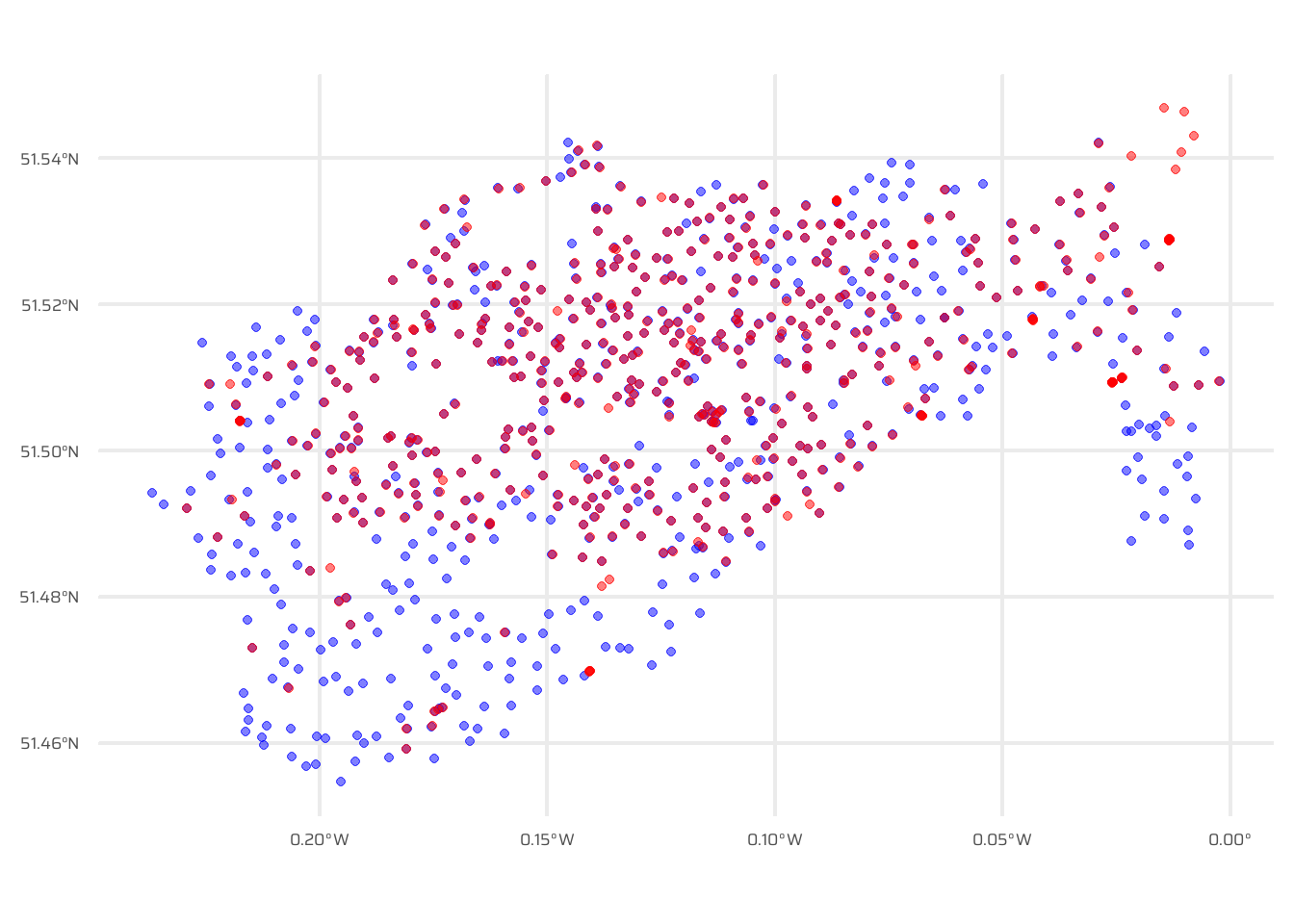
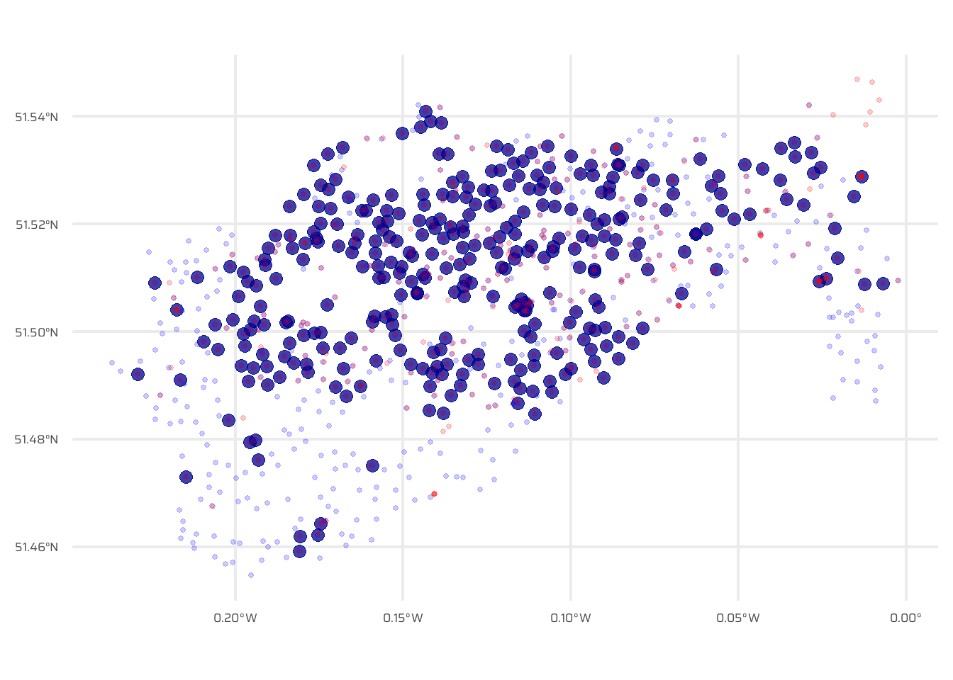
Figure 4 visualizes the spatial relationship between two datasets, cycle_hire and cycle_hire_osm, using a proximity filter. The st_filter() function from the sf package identifies points in the cycle_hire dataset that are within 10 meters of points in cycle_hire_osm, leveraging the st_is_within_distance predicate. The result is a subset of cycle_hire points, which are plotted using ggplot2. The plot includes:
Filtered
cycle_hirepoints (dark blue, fully opaque).All
cycle_hirepoints (dark blue, semi-transparent) for context.All
cycle_hire_osmpoints (red, semi-transparent) to show the proximity relationship.
Code
data("cycle_hire")
data("cycle_hire_osm")

ggplot() +
  geom_sf(
    data = cycle_hire,
    colour = "blue",
    alpha = 0.5
  ) +
  geom_sf(
    data = cycle_hire_osm,
    colour = "red",
    alpha = 0.5
  )
Code
# Official Cycle hire points with added info from OSM points within 10 metres
#
# cycle_hire |>
#   st_join(
#     cycle_hire_osm,
#     join = st_is_within_distance,
#     dist = units::set_units(10, "m")
#   )
Just checking, whether any of the two points in these two data sets exactly match. Well, they don’t!
st_intersects(cycle_hire, cycle_hire_osm, sparse = F) |> any()[1] FALSENow, in Figure 4, we highlight only those points of bike hire in the official data, which are within 10 metres of the OSM data. The important function here is st_filter() along with the argument .predicate = st_is_within_distance() and the argument dist = ... .
Code
# Plot only points which have a OSM point within 10 metres
cycle_hire |>
  st_filter(
    cycle_hire_osm,
    .predicate = st_is_within_distance,
    dist = units::set_units(10, "m")
  ) |>
  ggplot() +
  geom_sf(size = 3, alpha = 0.75, colour = "darkblue") +
  geom_sf(
    data = cycle_hire,
    alpha = 0.2,
    colour = "blue",
    size = 1
  ) +
  geom_sf(
    data = cycle_hire_osm,
    alpha = 0.2,
    colour = "red",
    size = 1
)4.2.7 Spatial Aggregation
- Spatial data aggregation condenses data into fewer rows by summarizing multiple values of a variable into a single value per grouping variable, similar to attribute data aggregation. Following two approaches exist: —
- Base R’s
aggregate(): Groups values based on spatial relationships and summarizes them with a specified function (e.g.,mean). - Tidyverse Approach (
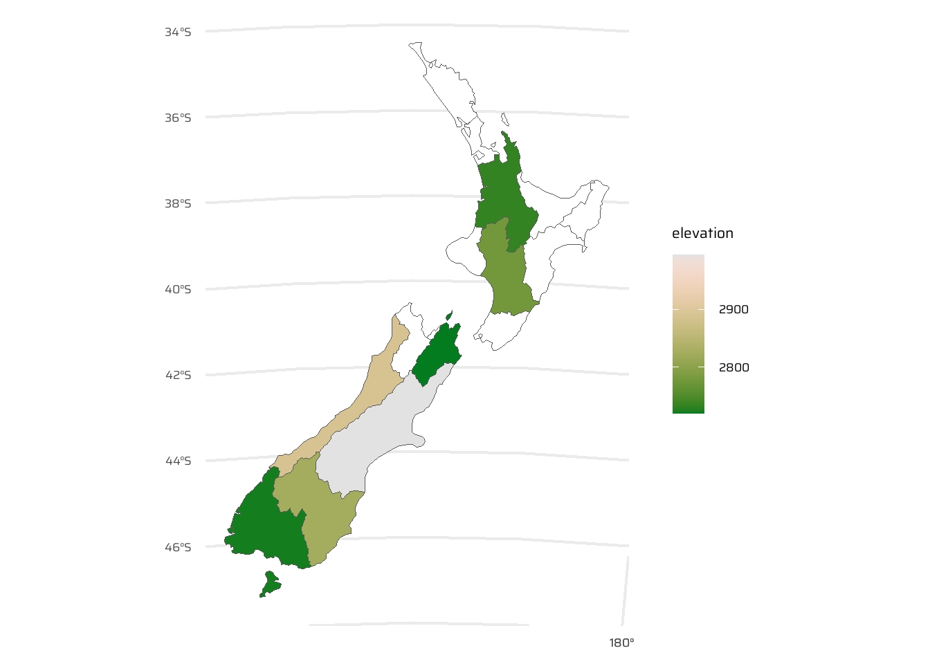
group_by()andsummarize()): Combinesst_join()with grouping and summarizing to perform spatial aggregation while allowing flexibility in function application and column naming. (This approach is better, as shown in Figure 5)
- Base R’s
- Output Differences:
aggregate()may result inNAfor unmatched regions.- Tidyverse methods preserve unmatched region names and allow for more flexible aggregation functions and output formatting.
- Functions like
median(),sd(), or other statistical summarizers can replacemean()for different aggregation purposes.
data("nz_height")
data("nz")

st_join(x = nz, y = nz_height) |>
  group_by(Name) |>
  summarise(elevation = mean(elevation, na.rm = T)) |>
  ggplot(
    mapping = aes(fill = elevation)
  ) +
  geom_sf() +
  paletteer::scale_fill_paletteer_c(
    "grDevices::Terrain 2",
    na.value = "white"
)4.2.8 Joining In-congruent Layers
Spatial congruence occurs when two layers (aggregating object
yand target objectx) share borders, enabling accurate spatial aggregation. Incongruence arises when no shared borders exist, complicating spatial operations.Example of Congruence:
- Administrative boundaries, such as districts made of smaller units, typically exhibit spatial congruence.
Issue with Incongruence:
- In-congruent layers, like sub-zones with differing borders from aggregating zones, result in inaccurate aggregations (e.g., centroids of sub-zones).
Solution: Areal Interpolation: Transfers values between areal units using:
- Simple area-weighted methods: Proportionally assigns values based on area overlap. This is implemented using
st_interpolate_aw(). - Advanced methods: Include algorithms like ‘pycnophylactic’ interpolation.
- Simple area-weighted methods: Proportionally assigns values based on area overlap. This is implemented using
Example Dataset:
- The spData package includes
incongruent(sub-zones) andaggregating_zones(larger zones). Thevaluecolumn inincongruentrepresents total regional income in million Euros, which must be aggregated intoaggregating_zones.
- The spData package includes
Implementation:
st_interpolate_aw():- The
st_interpolate_aw()function in the sf package performs areal-weighted interpolation of polygon data, allowing attributes from one spatial object (x) to be transferred to another (to) based on area overlap. Theextensiveargument determines whether attributes are spatially extensive (e.g., population, summed across areas) or spatially intensive (e.g., density, averaged). Additional options includekeep_NA(to retain or excludeNAfeatures) andna.rm(to remove features withNAattributes fromx). - Aggregated results depend on the variable type:
- Extensive variables: Values increase with area (e.g., total income).
- Intensive variables: Values remain constant irrespective of area (e.g., averages).
st_interpolate_aw()handles spatially extensive variables (e.g., total income) by summing values across areas.- In
st_interpolate_aw(), for spatially intensive variables (e.g., averages, percentages), setextensive = FALSEto use averages instead of sums. - Note: Warning messages indicate the assumption of uniform attribute distribution across areas.
- The
data("aggregating_zones")
data("incongruent")

# The two overall main zones for which the total income needs to be computed
aggregating_zones
Simple feature collection with 2 features and 3 fields
Geometry type: MULTIPOLYGON
Dimension: XY
Bounding box: xmin: 417686.2 ymin: 443703.6 xmax: 422959.3 ymax: 447036.8
Projected CRS: OSGB 1936 / British National Grid
geo_code geo_label geo_labelw geometry
5164 E02002332 Leeds 003 <NA> MULTIPOLYGON (((418731.9 44...
6631 E02002333 Leeds 004 <NA> MULTIPOLYGON (((419196.4 44...# The 9 smaller counties or districts or sub-units which are not
# congruent with the main zones
incongruentSimple feature collection with 9 features and 2 fields
Attribute-geometry relationships: aggregate (1), NA's (1)
Geometry type: MULTIPOLYGON
Dimension: XY
Bounding box: xmin: 417686.8 ymin: 443703 xmax: 422963 ymax: 446978
Projected CRS: OSGB 1936 / British National Grid
level value geometry
1 Incongruent 4.037919 MULTIPOLYGON (((420799.6 44...
2 Incongruent 5.014419 MULTIPOLYGON (((418664 4464...
3 Incongruent 4.933000 MULTIPOLYGON (((419964 4462...
4 Incongruent 5.120139 MULTIPOLYGON (((420368 4441...
5 Incongruent 6.548912 MULTIPOLYGON (((420419.8 44...
6 Incongruent 3.749791 MULTIPOLYGON (((421779 4451...
7 Incongruent 5.432837 MULTIPOLYGON (((419577 4464...
8 Incongruent 4.618049 MULTIPOLYGON (((417687.6 44...
9 Incongruent 5.956771 MULTIPOLYGON (((418859.3 44...# We are using extensive = TRUE, because our variable is
# total income, not average income
incongruent |>
# We need to keep only the numeric variable (and of course,
# the sticky geometry. Otherwise, R will not understand what
# to do with non-numeric columns)
select(value) |>
st_interpolate_aw(aggregating_zones, extensive = TRUE)Warning in st_interpolate_aw.sf(select(incongruent, value), aggregating_zones,
: st_interpolate_aw assumes attributes are constant or uniform over areas of xSimple feature collection with 2 features and 1 field
Attribute-geometry relationship: aggregate (1)
Geometry type: MULTIPOLYGON
Dimension: XY
Bounding box: xmin: 417686.2 ymin: 443703.6 xmax: 422959.3 ymax: 447036.8
Projected CRS: OSGB 1936 / British National Grid
value geometry
1 19.61613 MULTIPOLYGON (((418731.9 44...
2 25.66872 MULTIPOLYGON (((419196.4 44...4.3 Spatial operations on raster data
- Demonstrates advanced spatial raster operations.
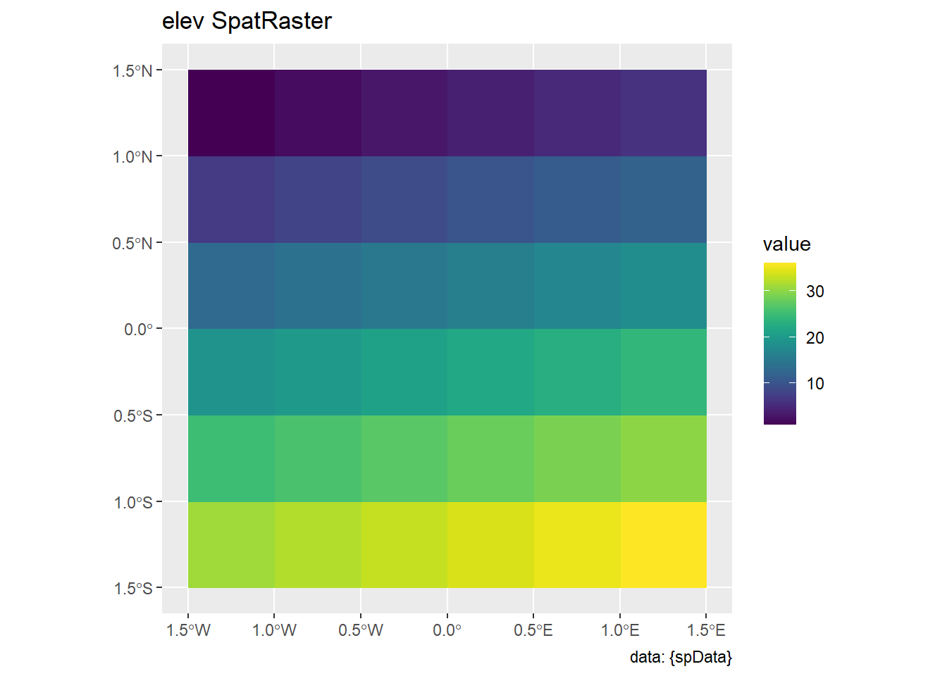
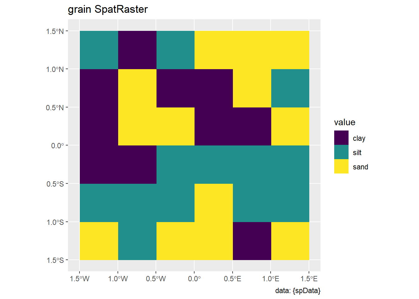
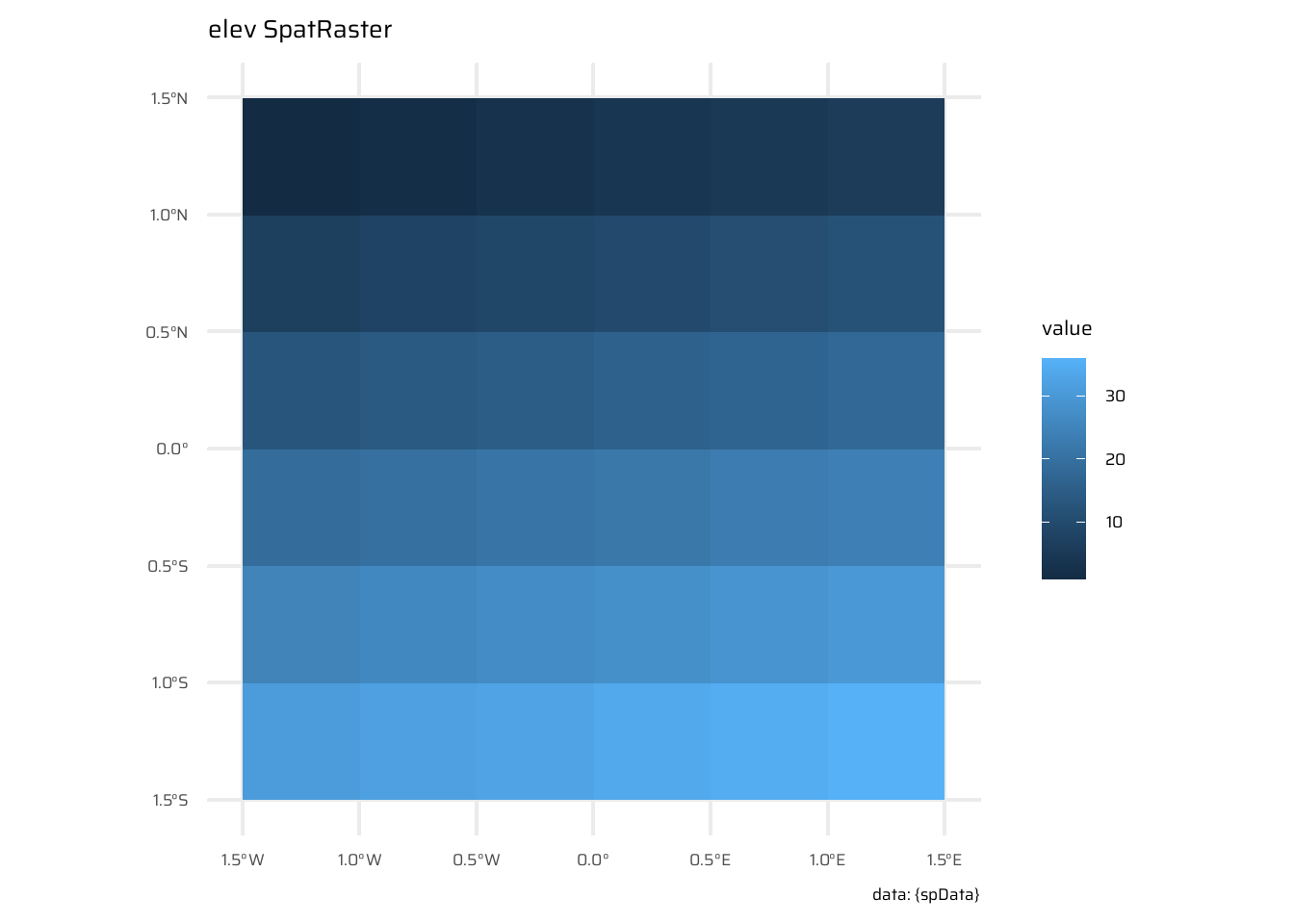
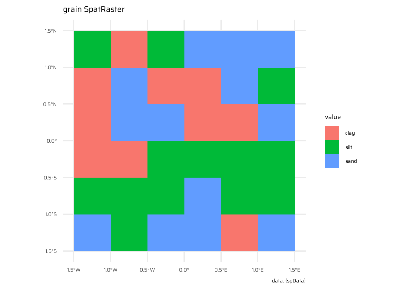
- Provides an alternative to manually creating datasets by accessing them from the
spDatapackage:elev: Represents elevation data.grain: Represents grain-related data.
elev <- rast(system.file("raster/elev.tif",
                        package = "spData"))

grain <- rast(system.file("raster/grain.tif",
                         package = "spData"))

# plot(elev)
# plot(grain)

ggplot() +
  geom_spatraster(data = elev) +
  labs(title = "elev SpatRaster", caption = "data: {spData}") +
  scale_fill_grass_c()


ggplot() +
  geom_spatraster(data = grain) +
  scale_fill_grass_d() +
labs(title = "grain SpatRaster", caption = "data: {spData}")4.3.1 Spatial subsetting
- Spatial subsetting allows extraction of raster data by location (coordinates) or spatial objects:
terra::extract(): Extracts raster values directly using coordinates. (Note: A function with the same name exists in the tidyverse, so be careful to add package name at start).
- Subsetting with another raster object:
- Use a secondary raster as a spatial mask to subset the primary raster, using
terra::crop(). - Example shown below: Subsetting
elevusing a smaller rasterclip_raster(defining a specific extent). - Two kinds of Spatial outputs from subsetting:
- Use the
dropargument with the[ ]operator to return subsetting results as raster objects. - Example: Subsets the first two cells of
elevwithelev[1:2, drop = FALSE], whereaselev[1:2]returns the cell values of first two cells only.
- Use the
- Use a secondary raster as a spatial mask to subset the primary raster, using
- Masking raster data with logical values:
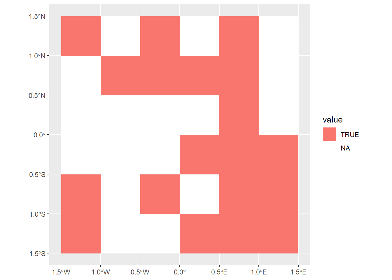
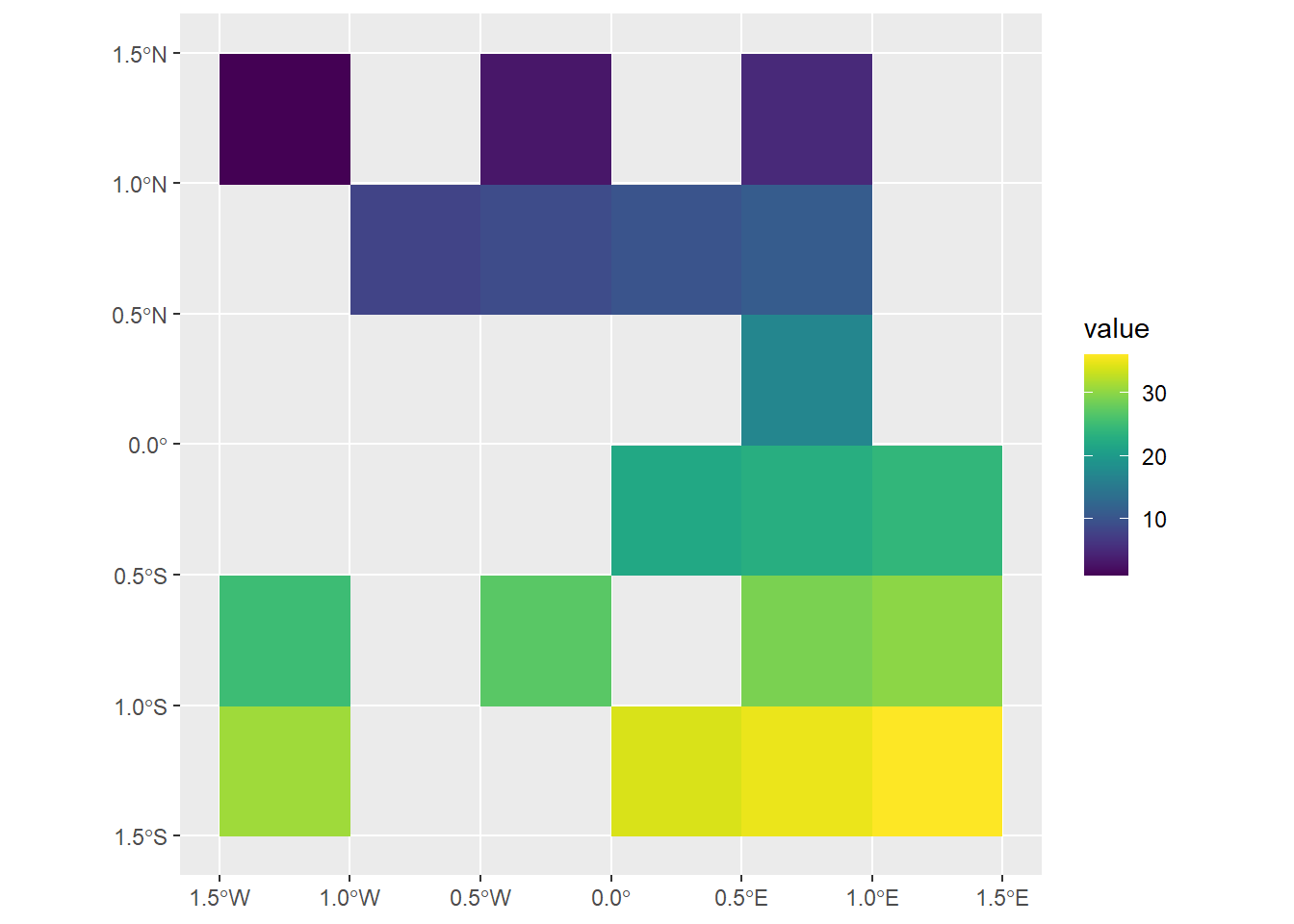
- Creates a raster mask (
rmask) with NA and TRUE values. - Masks the primary raster (
elev) to retain only values corresponding toTRUEin the mask using:[ ]operator - useTRUEandFALSE.mask()function - useTRUEandNA.
- Creates a raster mask (
- The
terra::crop()function extracts a subset of a raster or vector object based on a specified extent, defined using another spatial object orterra::ext(). It retains the input’s resolution and CRS, focusing analysis on a specific region. Commonly used for preprocessing large datasets, it pairs well withterra::mask()for refined cropping. - The
mask()function in theterrapackage applies a mask to a SpatRaster or SpatVector. It replaces values in a raster (x) withNA(or another value) where another raster or vector (mask) hasNAor specified mask values. It’s useful for filtering, clipping, or focusing on specific areas. - The
extract()function in the terra package retrieves values from aSpatRasterbased on specified locations or geometries. Locations can be points (as aSpatVector, matrix, or data frame), cell numbers, or spatial objects like polygons. It supports methods for exact or weighted extraction, interpolation, and summary statistics for extracted data. Key arguments include:x: TheSpatRasterto extract values fromy: Locations (e.g., points, polygons, or cell numbers) to extract values for.fun: Summarizes extracted data for polygons (e.g., mean, sum).cells/xy: Optionally return cell numbers or coordinates.weights/exact: Extract weighted or exact fractions for polygons.
# Let us extract some values from "elev" using coordinates
# I want to extract coordiantes of
coords_extract <- matrix(
  c(-1.2, -1.2,
    1.2, 1.2),
  ncol = 2,
  byrow = T
)

coords_extract
[,1] [,2]
[1,] -1.2 -1.2
[2,] 1.2 1.2elev |>
terra::extract(
y = coords_extract
) elev
1 31
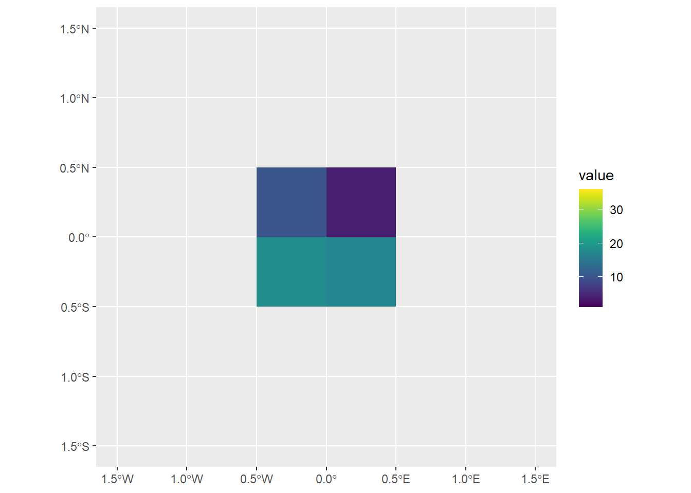
2 6# Let us create a new raster to clip the central four blocks of the elev raster
clip_raster <- rast(
xmin = -0.5, xmax = 0.5,
ymin = -0.5, ymax = 0.5,
resolution = 0.5,
vals = sample(1:25, 4)
)
# Extracting only the values
elev[clip_raster] elev
1 15
2 16
3 21
4 22# Explaining the meaning of argument drop = FALSE in the
# base R subsetting operator "[]"
elev[clip_raster] elev
1 15
2 16
3 21
4 22elev[clip_raster, drop = FALSE] class : SpatRaster
dimensions : 2, 2, 1 (nrow, ncol, nlyr)
resolution : 0.5, 0.5 (x, y)
extent : -0.5, 0.5, -0.5, 0.5 (xmin, xmax, ymin, ymax)
coord. ref. : lon/lat WGS 84 (EPSG:4326)
source(s) : memory
varname : elev
name : elev
min value : 15
max value : 22 # Using the {terra} approach: with the function terra::crop()
elev |>
terra::crop(clip_raster)class : SpatRaster
dimensions : 2, 2, 1 (nrow, ncol, nlyr)
resolution : 0.5, 0.5 (x, y)
extent : -0.5, 0.5, -0.5, 0.5 (xmin, xmax, ymin, ymax)
coord. ref. : lon/lat WGS 84 (EPSG:4326)
source(s) : memory
varname : elev
name : elev
min value : 15
max value : 22 # Creating a temporary_mask object
temporary_mask <- elev
values(temporary_mask) <- sample(c(NA, TRUE), 36,
replace = T)
elev |>
terra::mask(temporary_mask)class : SpatRaster
dimensions : 6, 6, 1 (nrow, ncol, nlyr)
resolution : 0.5, 0.5 (x, y)
extent : -1.5, 1.5, -1.5, 1.5 (xmin, xmax, ymin, ymax)
coord. ref. : lon/lat WGS 84 (EPSG:4326)
source(s) : memory
varname : elev
name : elev
min value : 1
max value : 36 ggplot() +
geom_spatraster(data = clip_raster) +
scale_x_continuous(limits = c(-1.5, 1.5)) +
scale_y_continuous(limits = c(-1.5, 1.5)) +
scale_fill_grass_c(limits = c(1, 36))
ggplot() +
geom_spatraster(data = temporary_mask) +
scale_fill_discrete(na.value = "white") +
scale_x_continuous(limits = c(-1.5, 1.5)) +
scale_y_continuous(limits = c(-1.5, 1.5))
ggplot() +
geom_spatraster(data = elev |> mask(temporary_mask)) +
scale_x_continuous(limits = c(-1.5, 1.5)) +
scale_y_continuous(limits = c(-1.5, 1.5)) +
scale_fill_grass_c(limits = c(1, 36))4.3.3 Local operations
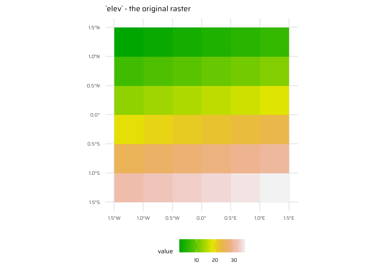
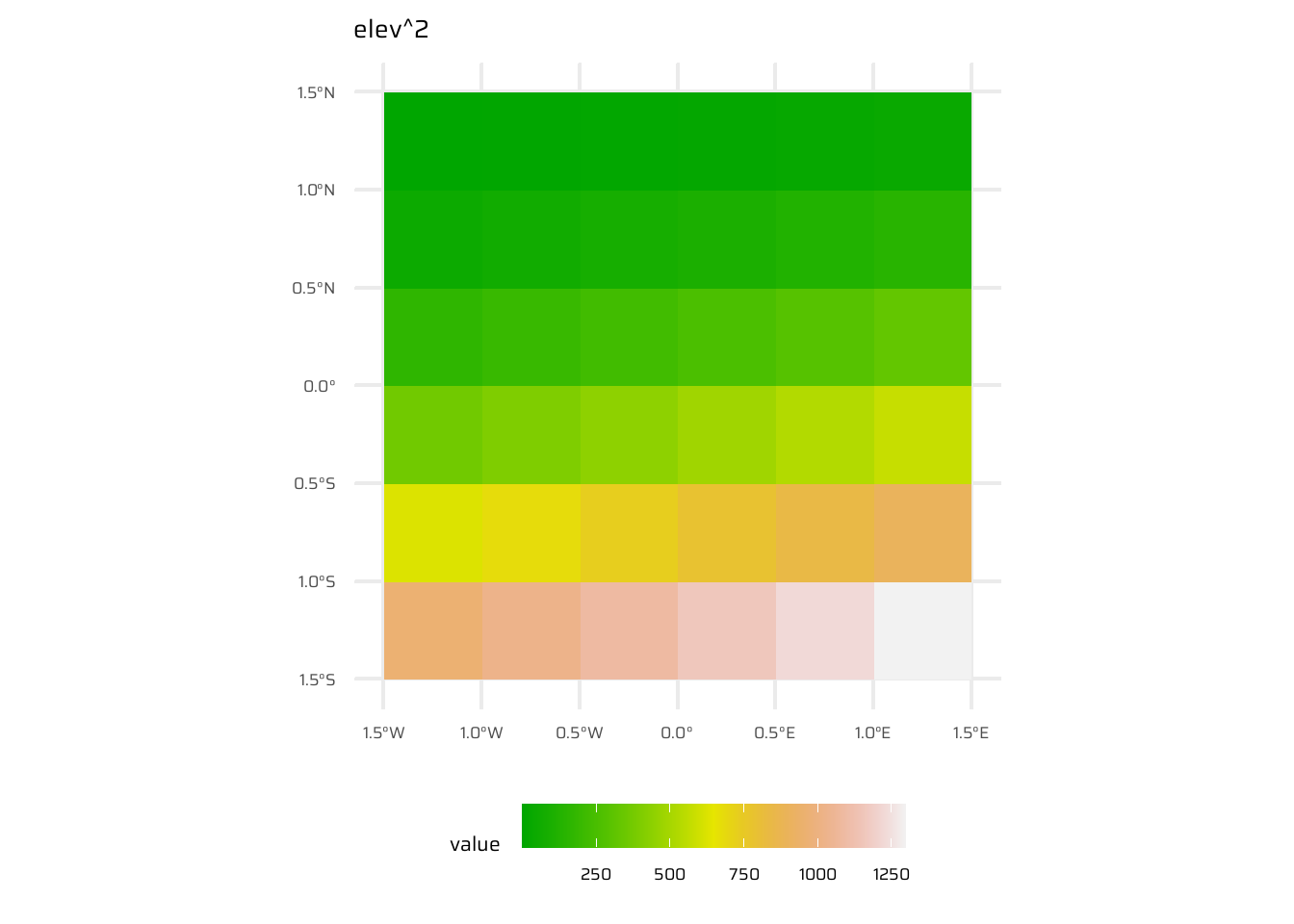
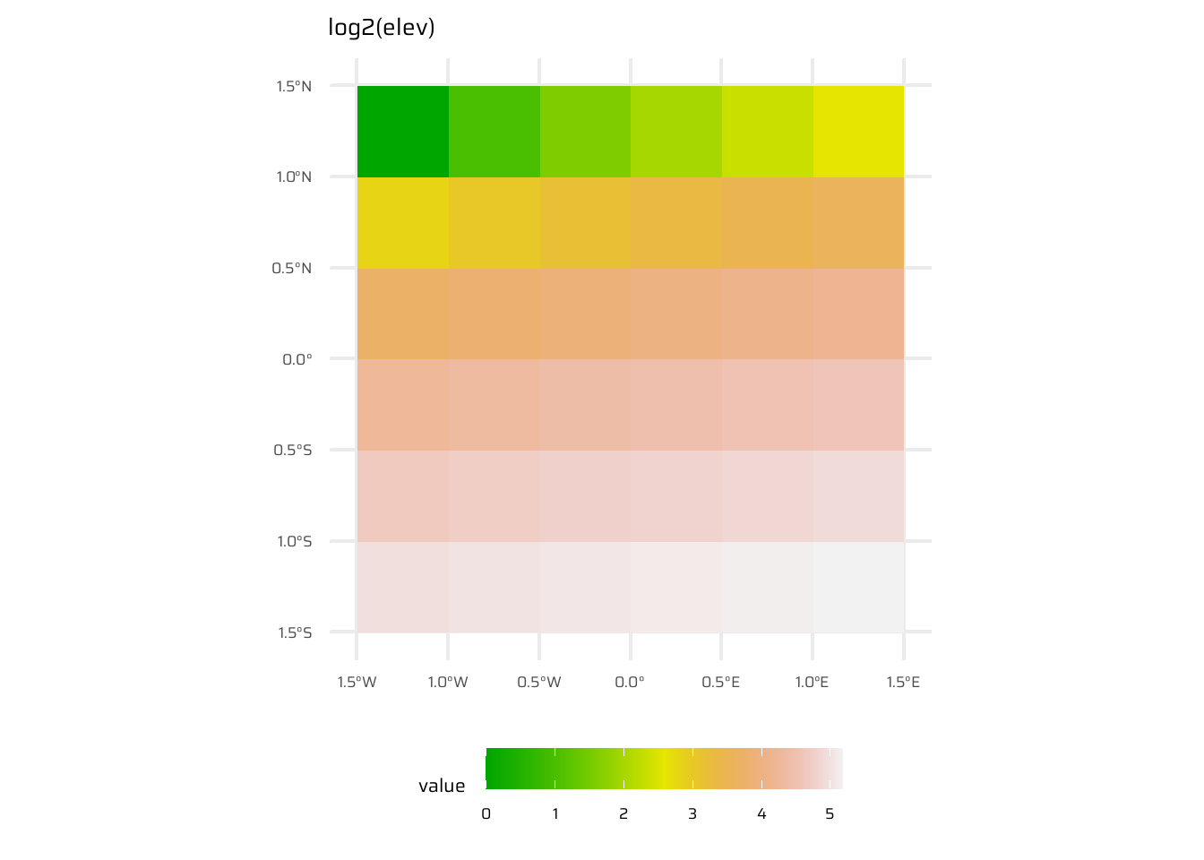
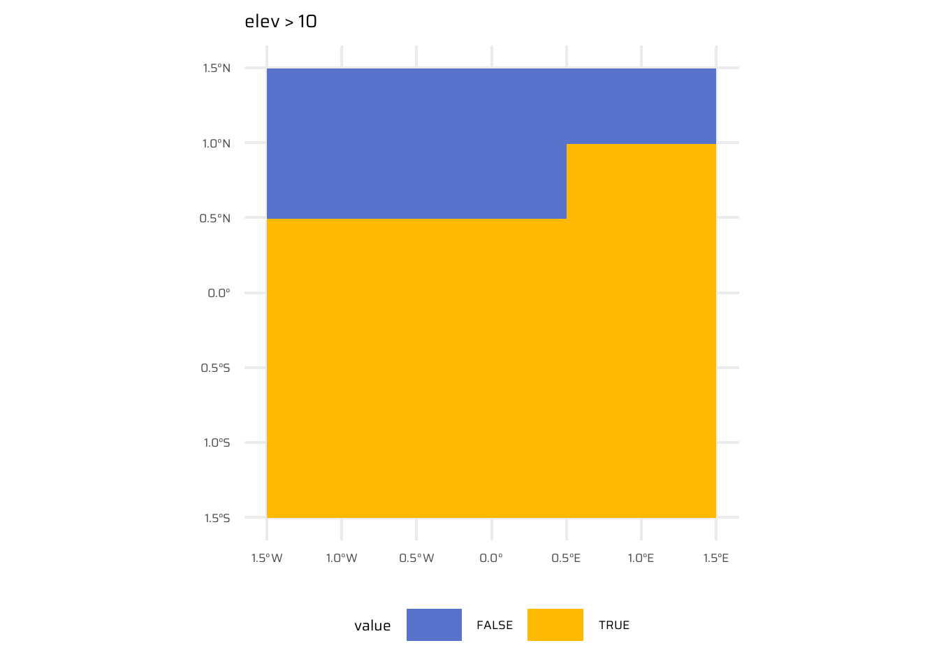
- Local operations are cell-by-cell operations performed on one or more raster layers. Includes operations like addition, subtraction, squaring, logical comparisons, and logarithmic transformations. Examples are shown in Figure 8
- Reclassification:
- Numeric values can be grouped into intervals (e.g., low, middle, high elevations).
- Use the
classify()function with a reclassification matrix to assign new values to defined ranges.
ggplot() +
  geom_spatraster(data = elev) +
  ggtitle("`elev` - the original raster") +
  paletteer::scale_fill_paletteer_c("grDevices::terrain.colors") +
  theme(legend.position = "bottom")

ggplot() +
  geom_spatraster(data = elev^2) +
  ggtitle("elev^2") +
  paletteer::scale_fill_paletteer_c("grDevices::terrain.colors") +
  theme(legend.position = "bottom",
        legend.key.width = unit(30, "pt"))

ggplot() +
  geom_spatraster(data = log2(elev)) +
  ggtitle("log2(elev)") +
  paletteer::scale_fill_paletteer_c("grDevices::terrain.colors") +
  theme(legend.position = "bottom",
        legend.key.width = unit(30, "pt"))


ggplot() +
  geom_spatraster(data = elev > 10) +
  ggtitle("elev > 10") +
 paletteer::scale_fill_paletteer_d("ggsci::alternating_igv") +
  theme(legend.position = "bottom",
legend.key.width = unit(30, "pt"))- Efficient alternatives for operations:
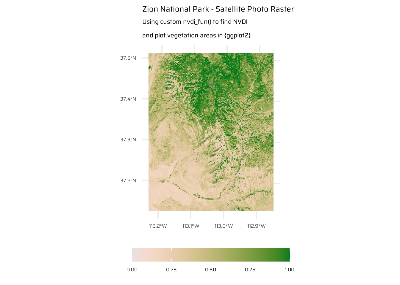
app(): Theapp()function in the{terra}package applies a user-defined or pre-existing function to each cell’s values of aSpatRaster, treating layers as columns in a matrix. Functions should return outputs divisible by the total cell count.tapp(): Thetapp()function in the{terra}package applies a function to subsets of layers in aSpatRastergrouped by an index. It allows for aggregation or summarization of layers based on grouping criteria such as indices, time periods (e.g., “years”, “months”), or custom functions.lapp(): Thelapp()function in the{terra}package applies a user-defined function to the layers of aSpatRasterorSpatRasterDataset, treating each layer as an argument to the function. The function must accept a vector of layer values and return a vector or matrix of the same or compatible size. This is useful for combining or transforming layers, such as performing arithmetic operations between them. An example oflapp()is the NDVI Calculation:- NDVI (Normalized Difference Vegetation Index) is a local operation to assess vegetation:
- Formula: (NIR - Red) / (NIR + Red).
- Calculated from satellite data (e.g., Landsat 8) with red and NIR bands.
- Positive NDVI values (> 0.2) indicate vegetation.
- Largest values correspond to dense forests, while lowest values are related to lakes and snowy areas.
- NDVI (Normalized Difference Vegetation Index) is a local operation to assess vegetation:
multi_rast = system.file("raster/landsat.tif", package = "spDataLarge")
multi_rast = rast(multi_rast)
# Rescale values to actual values (stored integers to save disk space)
multi_rast = (multi_rast * 0.0000275) - 0.2
# Remove negative values due to clouds etc.
multi_rast[multi_rast < 0] = 0
object.size(multi_rast)
1304 bytesndvi_fun = function(nir, red){
(nir - red) / (nir + red)
}
ndvi_rast = lapp(multi_rast[[c(4, 3)]], fun = ndvi_fun)
ggplot() +
geom_spatraster(
data = ndvi_rast,
mapping = aes(fill = lyr1)
) +
paletteer::scale_fill_paletteer_c(
"grDevices::Terrain 2",
direction = -1,
limits = c(0, 1),
oob = scales::squish
) +
labs(
title = "Zion National Park - Satellite Photo Raster",
subtitle = "Using custom nvdi_fun() to find NVDI\nand plot vegetation areas in {ggplot2}",
fill = NULL
) +
theme(
legend.position = "bottom",
legend.key.width = unit(40, "pt")
)4.3.4 Focal operations
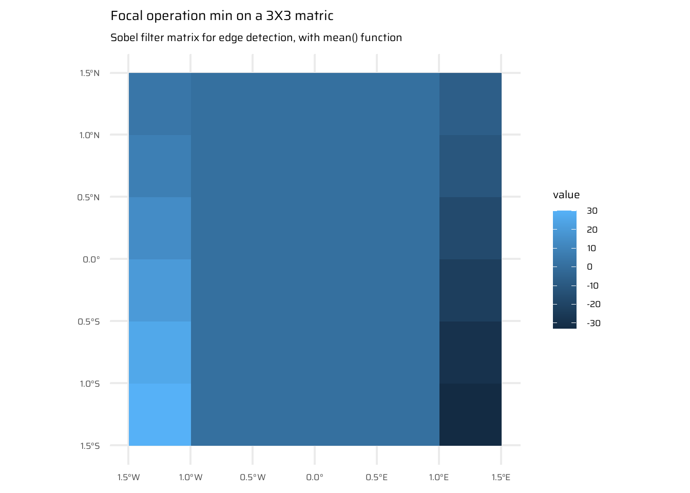
- Focal operations consider a central cell and its neighbours within a defined neighbourhood (kernel, filter, or moving window).
- Common neighbourhood size: 3x3 cells (central cell + 8 neighbours), but customizable sizes and shapes are supported.
- The operation aggregates values within the neighbourhood and assigns the result to the central cell, iterating across all cells.
- Implementation in R:
- Use the
focal()function to perform spatial filtering Figure 9. Parameters:w: Defines the weights of the moving window using a matrix, example in Figure 9 (c).fun: Specifies the aggregation function (e.g.,min,sum,mean,var), as in Figure 9 (b)
- Use the
- Applications:
- Spatial filtering or convolution for raster operations.
- Low-pass filters:
- Use the mean function to smooth and reduce extreme values.
- For categorical data, replace the mean with the mode (most common value).
- High-pass filters:
- Enhance features using methods like Laplace or Sobel filters (e.g., line detection).
- Terrain processing:
- Compute topographic characteristics like slope, aspect, and flow directions using focal functions.
ggplot() +
  geom_spatraster(data = elev) +
  labs(title = "elev SpatRaster", caption = "data: {spData}")

ggplot() +
  geom_spatraster(
    data = elev |>
        terra::focal(
        w = matrix(rep(1, 9), 3, 3),
        fun = min
      )
  ) +
  labs(title = "Focal operation min on a 3X3 matric",
       subtitle = "Simple min() function with na.rm = FALSE")

ggplot() +
  geom_spatraster(
    data = elev |>
        terra::focal(
        # Sobel filters (for edge detection):
        w = matrix(c(-1,-2,-1,0,0,0,1,2,1), nrow = 3),
        fun = mean,
        na.rm = TRUE
      )
  ) +
  labs(
    title = "Focal operation min on a 3X3 matric",
    subtitle = "Sobel filter matrix for edge detection, with mean() function"
)4.3.5 Zonal operations
- Zonal operations aggregate raster cell values based on zones defined by a second raster with categorical values. Unlike focal operations, zones in zonal operations do not require neighboring cells to be adjacent.
- Key Characteristics:
- The
zonal()function in the terra package computes zonal statistics by summarizing the values of aSpatRasterfor each “zone” defined by anotherSpatRaster. It applies a specified function (fun, e.g., mean, sum) to aggregate the data for each zone. - The result is typically a summary table, grouped by zones. Zones are defined by a secondary raster.
- Optional Output: A raster with calculated statistics for each zone can be generated by setting
as.raster = TRUE.
- The
- Usage:
- Ideal for summarizing raster values based on irregularly spread categorical zones.
- Commonly used in land classification, soil analysis, and other spatial analyses where zones are pre-defined.
ggplot() +
  geom_spatraster(data = elev) +
  labs(title = "elev SpatRaster", caption = "data: {spData}")


ggplot() +
  geom_spatraster(data = grain) +
labs(title = "grain SpatRaster", caption = "data: {spData}")elev |>
terra::zonal(
z = grain,
fun = mean
) |>
as_tibble()# A tibble: 3 × 2
grain elev
<chr> <dbl>
1 clay 14.8
2 silt 21.2
3 sand 18.74.3.6 Global operations and distances
- Global operations consider the entire raster dataset as a single zone.
- Common operations include:
- Descriptive statistics: Minimum, maximum, etc.
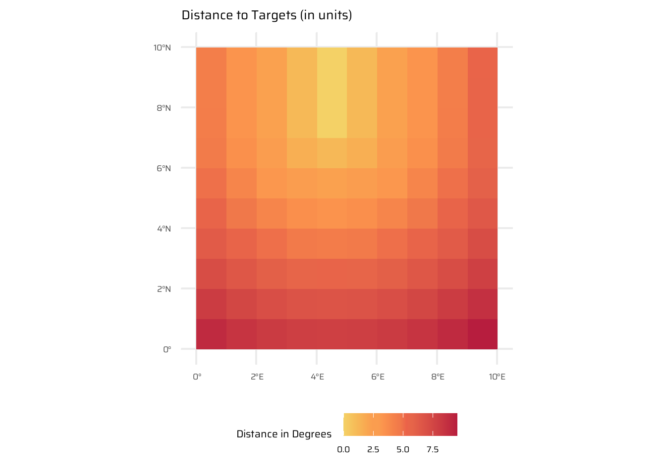
- Distance calculations: Compute distance from each cell to a target cell using
terra::distance(). Theterra::distance()function calculates the shortest distance from each cell in a raster to a set of target cells, which are identified based on a condition (e.g., where raster values are non-NA, equal to a specific value, or greater than a threshold). This is useful for spatial analysis, such as finding proximity to certain features or zones in a raster. - Weighted distances: Factor in additional variables, such as elevation, to modify distance calculations.
- Visibility and viewshed analysis: Assess visible areas from a specific point.
- Applications:
- Distance to coastlines or other target areas.
- Topography-aware distance calculations.
- Advanced spatial modeling like visibility analysis.
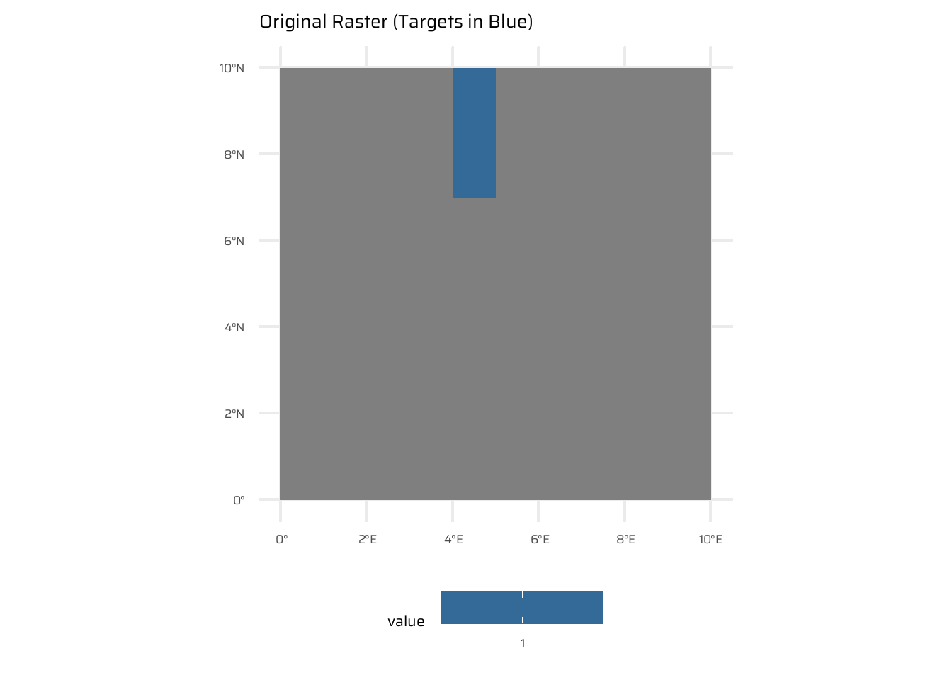
# Create a sample SpatRaster
r <- rast(ncols = 10, nrows = 10,
          xmin = 0, xmax = 10,
          ymin = 0, ymax = 10)
values(r) <- NA
values(r)[c(5, 15, 25)] <- 1  # Assign specific cells as targets

# Compute the distance to the non-NA cells
dist_raster <- distance(r)
|---------|---------|---------|---------|
=========================================
dist_raster <- dist_raster * 1e-5# View the raster
ggplot() +
geom_spatraster(data = r) +
labs(title = "Original Raster (Targets in Blue)") +
theme(
legend.position = "bottom"
)
# View the distance raster
ggplot() +
geom_spatraster(data = dist_raster) +
labs(title = "Distance to Targets (in units)",
fill = "Distance in Degrees") +
paletteer::scale_fill_paletteer_c("ggthemes::Red-Gold") +
theme(legend.position = "bottom")4.3.7 Map algebra counterparts in vector processing
- Equivalence between raster and vector operations:
- Distance raster (global operation) ≈ Buffer operation (vector) (Section 5.2.5).
- Raster reclassification ≈ Dissolving vector boundaries (Section 4.2.5).
- Raster overlay with masks ≈ Vector clipping (Section 5.2.5).
- Zonal operations ≈ Aggregating vector geometries by zones.
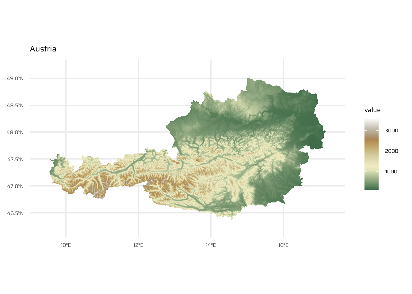
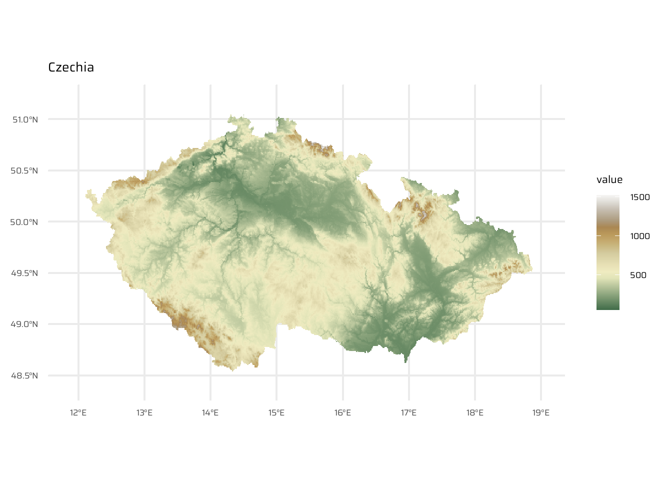
4.3.8 Merging rasters
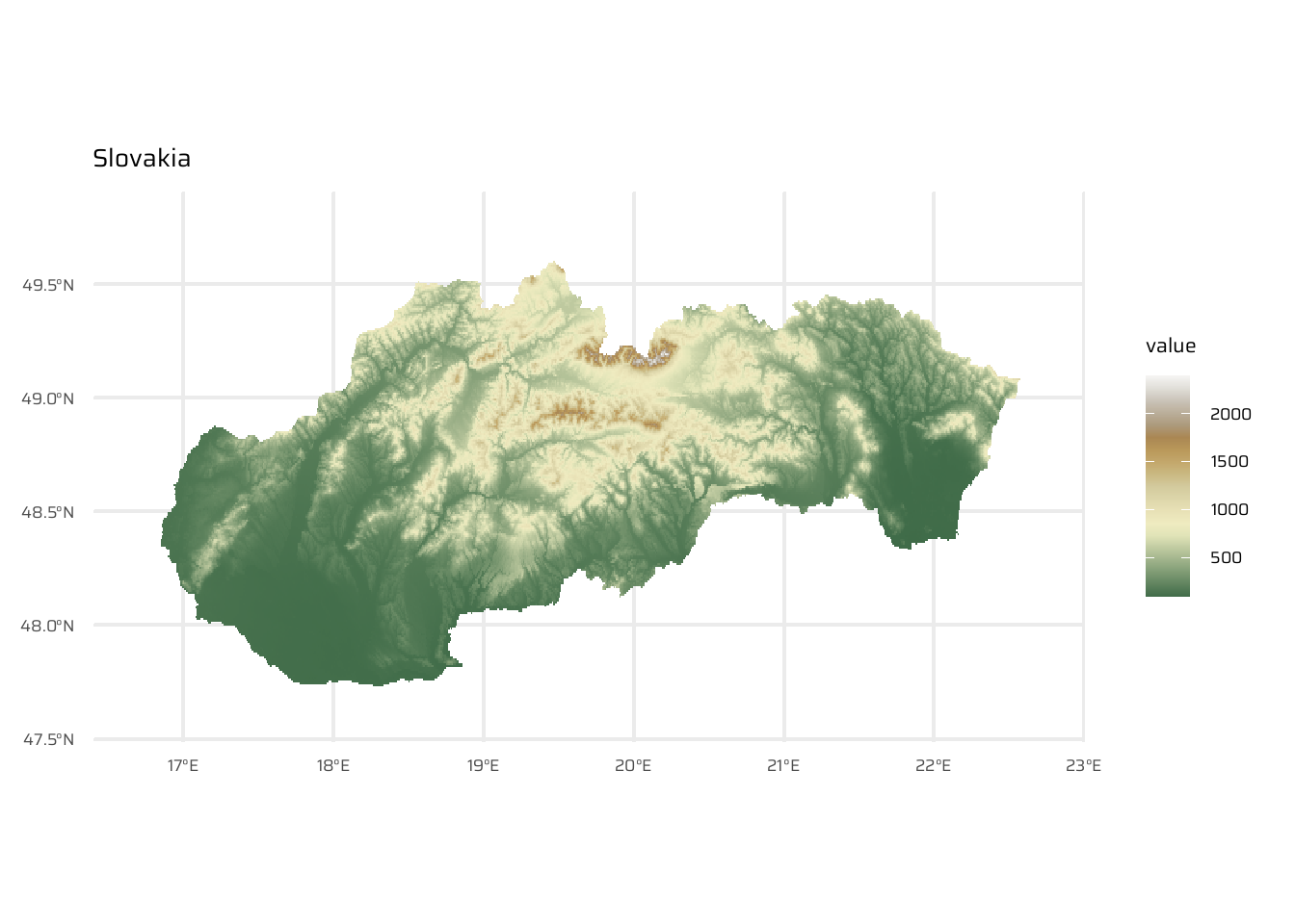
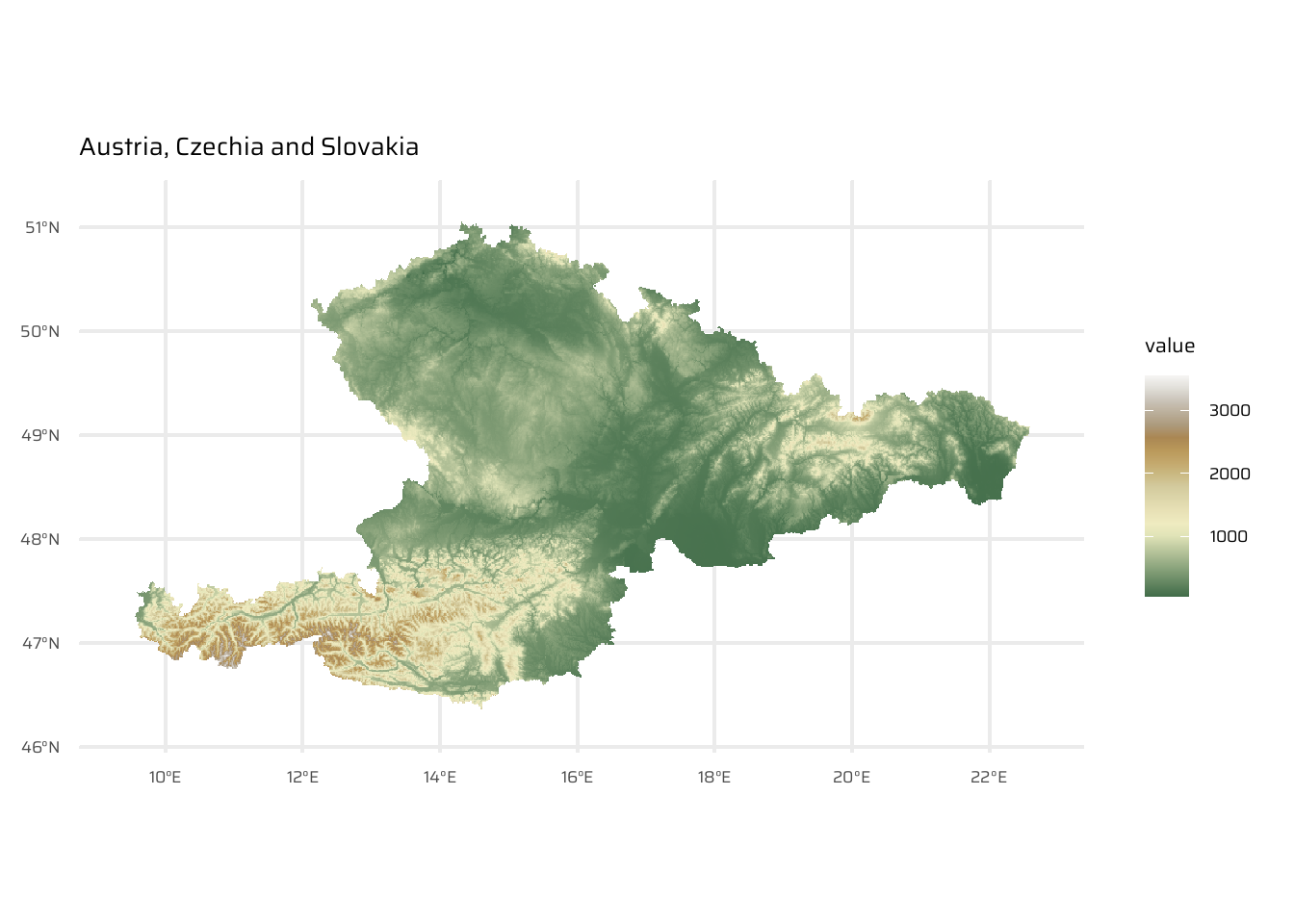
Combines multiple raster datasets into a single raster. Often required for datasets spanning multiple spatial scenes (e.g., satellite imagery, elevation data).
merge():- Places rasters side by side.
- For overlapping areas, prioritizes values from the first raster.
aut <- geodata::elevation_30s(country = "AUT", path = tempdir())
ggplot() +
  geom_spatraster(data = aut) +
  scale_fill_wiki_c() +
  ggtitle("Austria")
cze <- geodata::elevation_30s(country = "CZE", path = tempdir())
ggplot() +
geom_spatraster(data = cze) +
scale_fill_wiki_c() +
ggtitle("Czechia")svk <- geodata::elevation_30s(country = "SVK", path = tempdir())
ggplot() +
geom_spatraster(data = svk) +
scale_fill_wiki_c() +
ggtitle("Slovakia")aut_cze_svk <- aut |>
merge(svk) |>
merge(cze)
ggplot() +
geom_spatraster(data = aut_cze_svk) +
scale_fill_wiki_c() +
ggtitle("Austria, Czechia and Slovakia")mosaic():- Handles overlaps by applying a function (e.g., mean) to the overlapping area.
- Helps smooth visible borders but may not eliminate them entirely.
4.4 Exercises
E1.
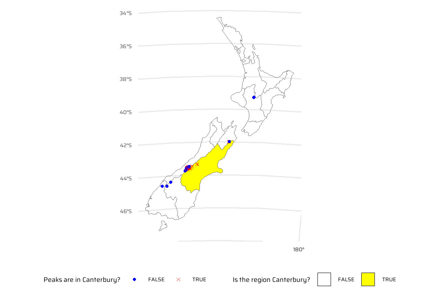
It was established in Section 4.2 that Canterbury was the region of New Zealand containing most of the 101 highest points in the country. How many of these high points does the Canterbury region contain?
Canterbury contains 70 of these high points.
data("nz")
data("nz_height")

nz_height |>
  st_intersection(
    nz |> filter(Name == "Canterbury")
  ) |>
  nrow()
[1] 70Bonus: plot the result using the plot() function to show all of New Zealand, canterbury region highlighted in yellow, high points in Canterbury represented by red crosses (hint: pch = 7) and high points in other parts of New Zealand represented by blue circles. See the help page ?points for details with an illustration of different pch values.
nz_height |>
  mutate(
    in_canterbury = nz_height |>
      st_intersects(
        nz |> filter(Name == "Canterbury"),
        sparse = FALSE
      )
  ) |>
  ggplot() +
  geom_sf(
    data = nz |> mutate(fill_var = Name == "Canterbury"),
    mapping = aes(fill = fill_var)
  ) +
  geom_sf(
    mapping = aes(shape = in_canterbury, colour = in_canterbury)
  ) +
  scale_shape_manual(values = c(16, 4)) +
  scale_colour_manual(values = c("blue", "red")) +
  scale_fill_manual(values = c("transparent", "yellow")) +
  labs(
    fill = "Is the region Canterbury?",
    colour = "Peaks are in Canterbury?",
    shape = "Peaks are in Canterbury?"
  ) +
  theme(legend.position = "bottom")
E2.
Which region has the second highest number of nz_height points, and how many does it have?
The region with second highest number of nz_height points is West Coast. It has 22 such points.
nz_height |>
  st_join(nz) |>
  st_drop_geometry() |>
  group_by(Name) |>
  count()
# A tibble: 7 × 2
# Groups: Name [7]
Name n
<chr> <int>
1 Canterbury 70
2 Manawatu-Wanganui 2
3 Marlborough 1
4 Otago 2
5 Southland 1
6 Waikato 3
7 West Coast 22E3.
Generalizing the question to all regions: how many of New Zealand’s 16 regions contain points which belong to the top 101 highest points in the country? Which regions?
- Bonus: create a table listing these regions in order of the number of points and their name.
Seven (7) regions of New Zealand contain points which belong to top 101 highest points in the country. The table is shown below.
nz_height |>
  st_join(nz) |>
  st_drop_geometry() |>
  group_by(Name) |>
  count(name = "Number of points", sort = T) |>
  ungroup() |>
  mutate(`S.No.` = row_number()) |>
  relocate(`S.No.`) |>
  gt::gt() |>
  gtExtras::gt_theme_538() |>
  gt::tab_header(
    title = "Number of highest points in each region of New Zealand"
)| Number of highest points in each region of New Zealand | ||
|---|---|---|
| S.No. | Name | Number of points |
| 1 | Canterbury | 70 |
| 2 | West Coast | 22 |
| 3 | Waikato | 3 |
| 4 | Manawatu-Wanganui | 2 |
| 5 | Otago | 2 |
| 6 | Marlborough | 1 |
| 7 | Southland | 1 |
Test your knowledge of spatial predicates by finding out and plotting how US states relate to each other and other spatial objects.
E4.
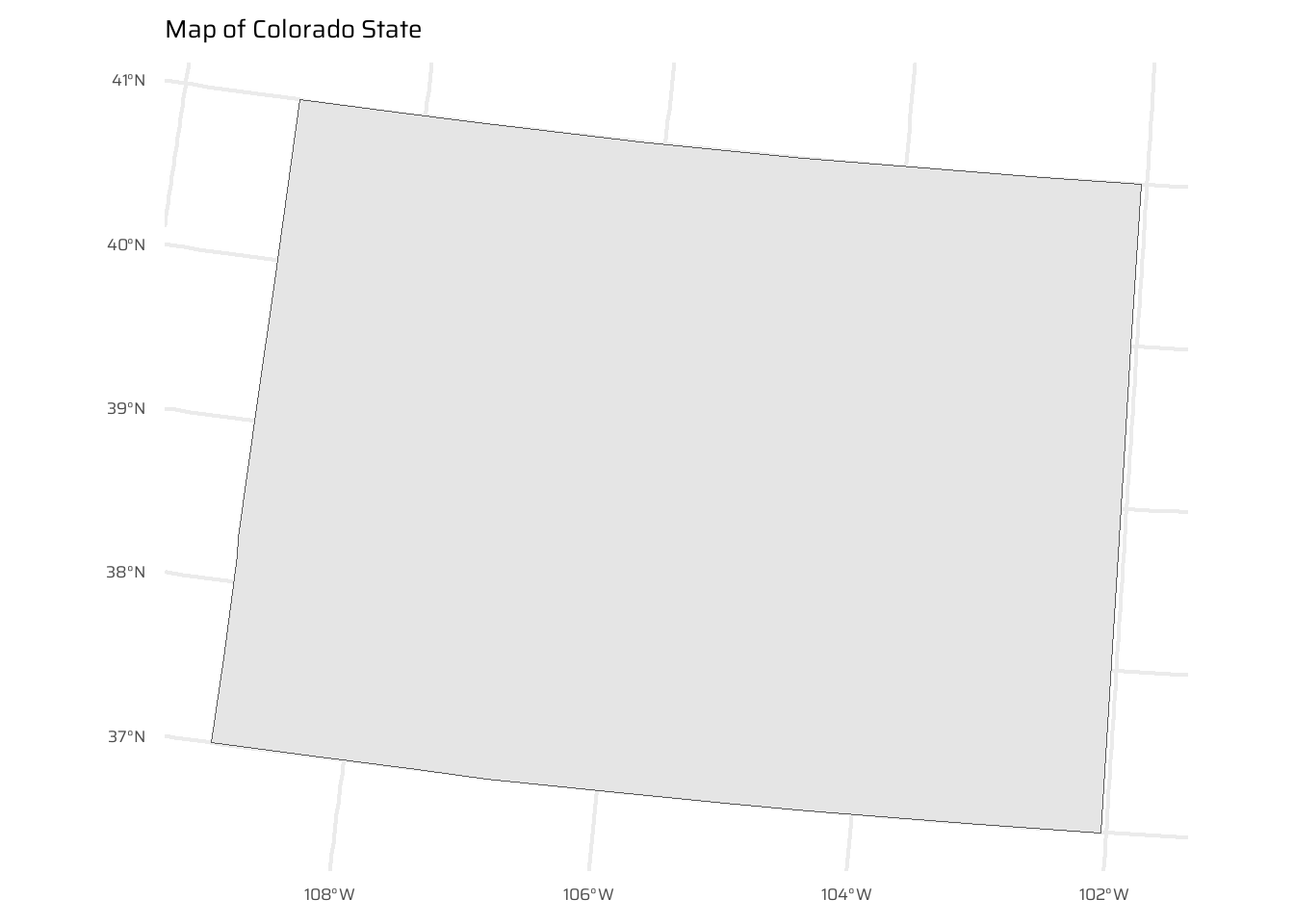
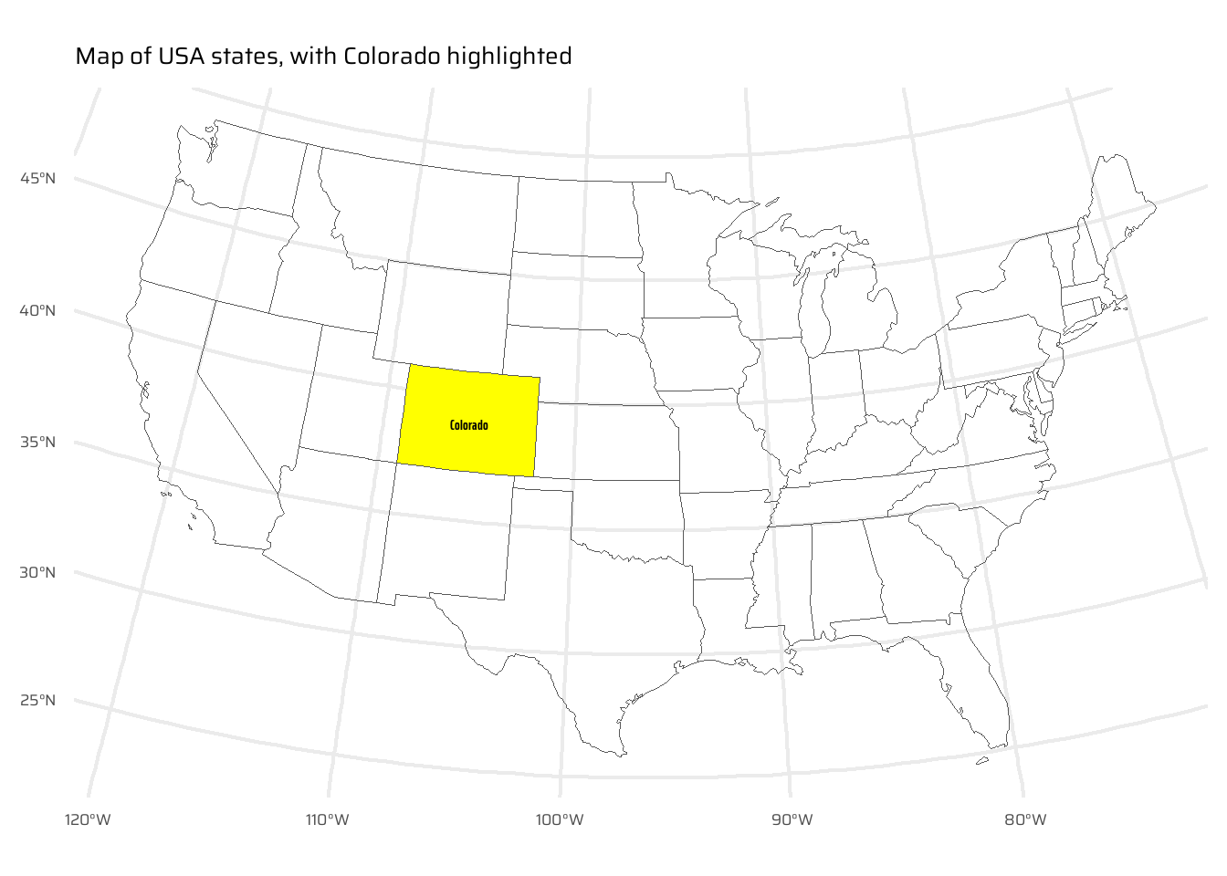
The starting point of this exercise is to create an object representing Colorado state in the USA. Do this with the command colorado = us_states[us_states$NAME == "Colorado",] (base R) or with the filter() function (tidyverse) and plot the resulting object in the context of US states.
data("us_states")

colorado <- us_states |>
  filter(NAME == "Colorado")

ggplot() +
  geom_sf(data = colorado) +
  ggtitle("Map of Colorado State") +
  coord_sf(
    crs = "EPSG:5070"
)- Create a new object representing all the states that geographically intersect with Colorado and plot the result (hint: the most concise way to do this is with the subsetting method
[).
ggplot() +
  geom_sf(
    data = us_states,
    fill = "transparent"
  ) +
  geom_sf(
    data = colorado,
    fill = "yellow"
  ) +
  geom_sf_text(
    data = colorado,
    mapping = aes(
      label = NAME
    ),
    family = "caption_font",
    fontface = "bold"
  ) +
  coord_sf(
    crs = "EPSG:5070"
  ) +
  labs(
    x = NULL, y = NULL,
    title = "Map of USA states, with Colorado highlighted"
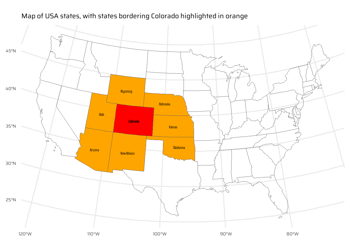
)- Create another object representing all the objects that touch (have a shared boundary with) Colorado and plot the result (hint: remember you can use the argument
op = st_intersectsand other spatial relations during spatial subsetting operations in base R).
bordering <- us_states |>
  mutate(
    border_colorado = as_vector(
      as_vector(
        us_states |>
        st_intersects(colorado, sparse = FALSE)
      )
    )
  )

ggplot() +
  geom_sf(
    data = bordering,
    mapping = aes(
      fill = border_colorado
    )
  ) +
  scale_fill_manual(
    values = c("transparent", "orange")
  ) +
  geom_sf_text(
    data = filter(bordering, border_colorado),
    mapping = aes(
      label = NAME
    ),
    family = "caption_font"
  ) +
  geom_sf(
    data = colorado,
    fill = "red"
  ) +
  geom_sf_text(
    data = colorado,
    mapping = aes(
      label = NAME
    ),
    family = "caption_font",
    fontface = "bold"
  ) +
  coord_sf(
    crs = "EPSG:5070"
  ) +
  labs(
    x = NULL, y = NULL,
    title = "Map of USA states, with states bordering Colorado highlighted in orange"
  ) +
  theme(
    legend.position = "none"
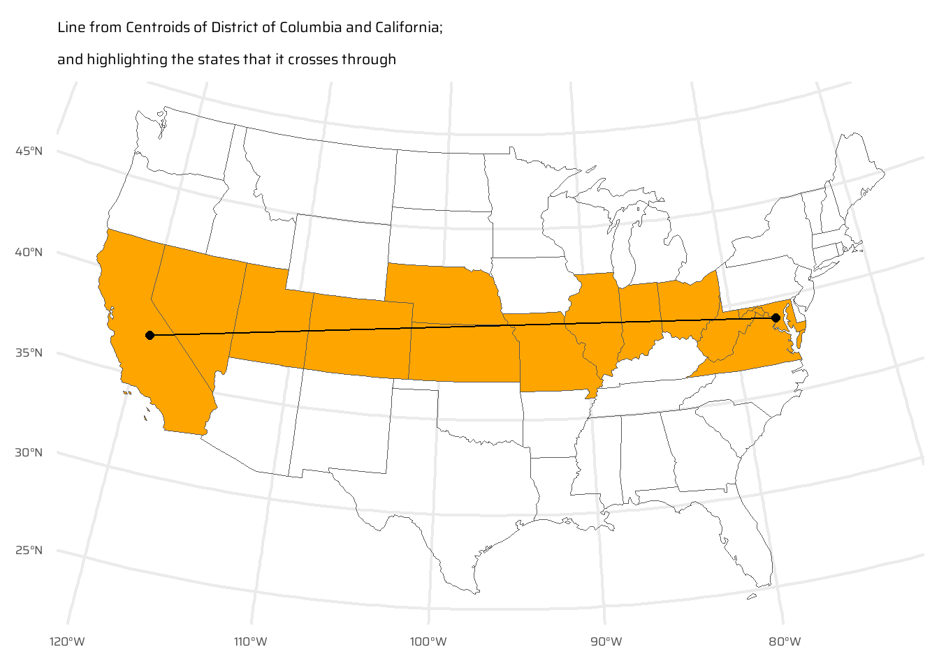
)- Bonus: create a straight line from the centroid of the District of Columbia near the East coast to the centroid of California near the West coast of the USA (hint: functions
st_centroid(),st_union()andst_cast()described in Chapter 5 may help) and identify which states this long East-West line crosses.
wdc_centre <- st_centroid(
  us_states |> filter(NAME == "District of Columbia")
) |>
  pull(geometry)

cal_centre <- st_centroid(
  us_states |> filter(NAME == "California")
) |>
  pull(geometry)

straight_line <- st_union(
  wdc_centre,
  cal_centre
) |>
  st_cast(
    "LINESTRING"
  )

us_states |>
  mutate(
    on_the_way = as_vector(
      st_intersects(
        us_states,
        straight_line,
        sparse = FALSE
      )
    )
  ) |>
  ggplot() +
  geom_sf(
    mapping = aes(
      fill = on_the_way
    )
  ) +
  scale_fill_manual(
    values = c("transparent", "orange")
  ) +
  geom_sf(
    data = straight_line,
    linewidth = 0.5
  ) +
  geom_sf(
    data = cal_centre,
    size = 2
  ) +
  geom_sf(
    data = wdc_centre,
    size = 2
  ) +
  coord_sf(
    crs = "EPSG:5070"
  ) +
  labs(
    subtitle = "Line from Centroids of District of Columbia and California;\nand highlighting the states that it crosses through"
  ) +
  theme(
    legend.position = "none"
  )
E5.
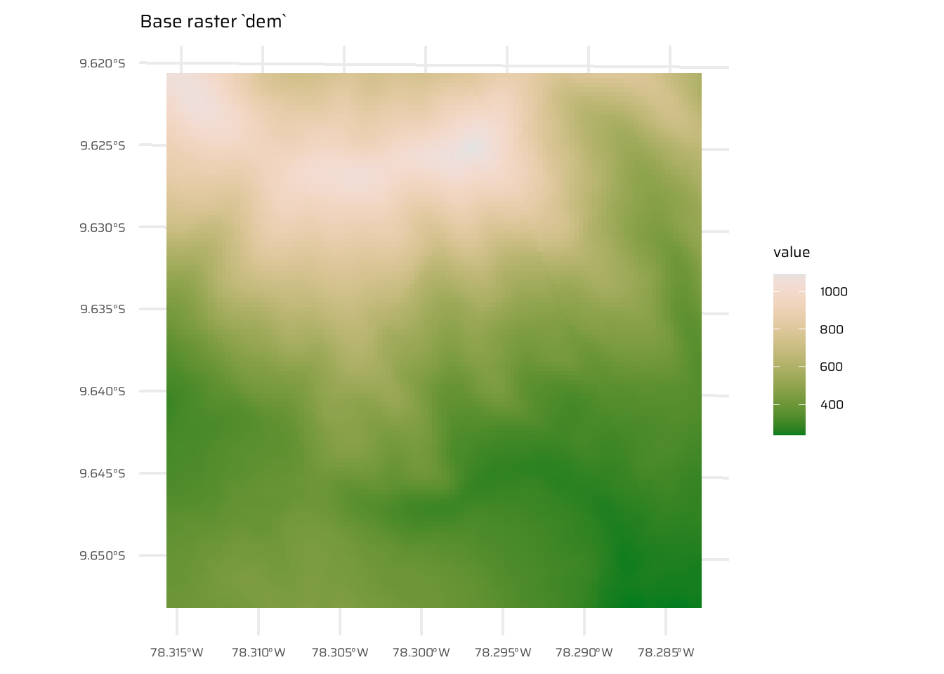
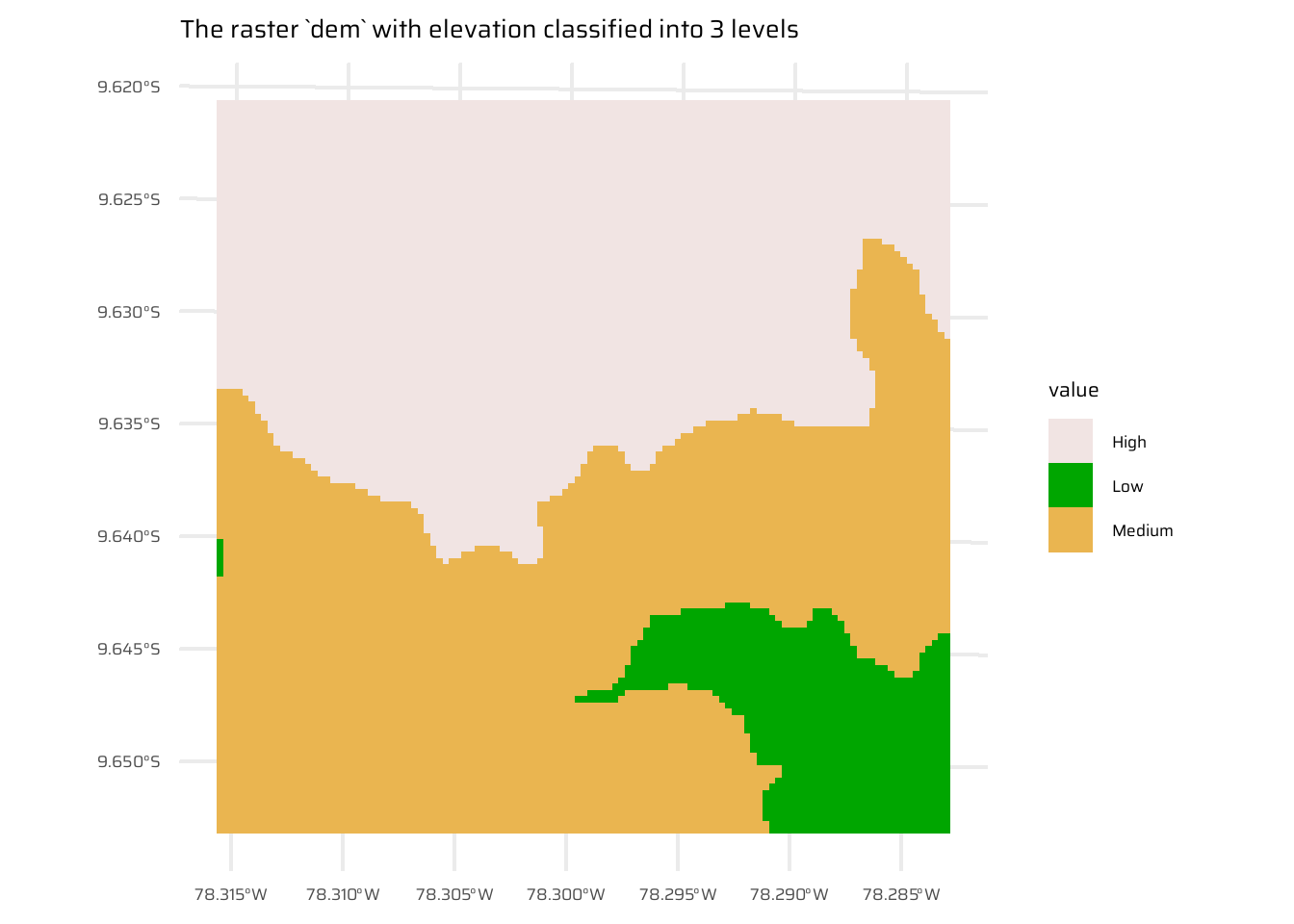
Use dem = rast(system.file("raster/dem.tif", package = "spDataLarge")), and reclassify the elevation in three classes: low (<300), medium and high (>500). Secondly, read the NDVI raster (ndvi = rast(system.file("raster/ndvi.tif", package = "spDataLarge"))) and compute the mean NDVI and the mean elevation for each altitudinal class.
dem <- rast(system.file("raster/dem.tif", package = "spDataLarge"))

ggplot() +
  geom_spatraster(data = dem) +
  paletteer::scale_fill_paletteer_c("grDevices::Terrain 2") +
  ggtitle("Base raster `dem`")

dem1 <- dem

values(dem1) <- values(dem) |>
  as_tibble() |>
  mutate(
    dem_class = case_when(
      dem < 300 ~ "Low",
      dem > 500 ~ "High",
      .default = "Medium"
    )
  ) |>
  pull(dem_class)

ggplot() +
  geom_spatraster(data = dem1) +
  scale_fill_manual(values = c("#F1E4E3FF", "#00A600FF", "#EAB550FF")) +
ggtitle("The raster `dem` with elevation classified into 3 levels")ndvi <- rast(system.file("raster/ndvi.tif", package = "spDataLarge"))
tibble(
elevation_class = values(dem1),
elevation = values(dem),
ndvi = values(ndvi)
) |>
group_by(elevation_class) |>
summarise(
mean_elevation = mean(elevation),
mean_ndvi = mean(ndvi)
) |>
gt::gt() |>
gt::fmt_number(
columns = c(mean_elevation, mean_ndvi)
) |>
gt::cols_label_with(fn = snakecase::to_title_case) |>
gt::tab_header(
title = "Mean elevation and NDVI for each altitude class"
) |>
gtExtras::gt_theme_538()| Mean elevation and NDVI for each altitude class | ||
|---|---|---|
| Elevation Class | Mean Elevation | Mean Ndvi |
| 1 | 765.22 | −0.21 |
| 2 | 273.79 | −0.36 |
| 3 | 391.61 | −0.29 |
E6.
Apply a line detection filter to rast(system.file("ex/logo.tif", package = "terra")). Plot the result. Hint: Read ?terra::focal().
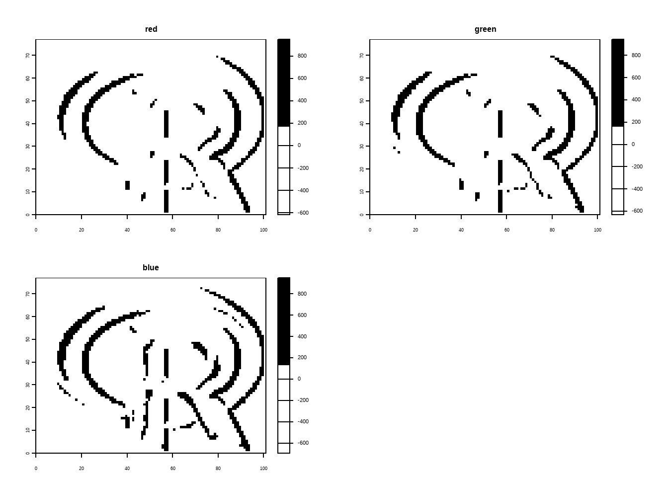
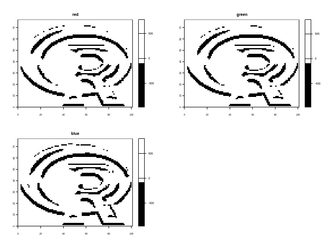
The code below demonstrates edge detection on a raster image using Sobel filters with the {terra} package in R. The Sobel filters, represented as matrices fx and fy, are defined for detecting edges in horizontal and vertical directions, respectively. The focal() function applies these filters to the raster image, performing convolution to emphasize areas of rapid intensity change (edges). The processed images are then plotted, one showing horizontal edges (filtered with fx) in black and white, and the other showing vertical edges (filtered with fy) in white and black. This illustrates how Sobel filters can be used for edge detection in spatial raster data.
logo <- rast(system.file("ex/logo.tif", package = "terra"))

plot(logo)

# Sobel filters (for edge detection):
fx <- matrix(c(-1,-2,-1,0,0,0,1,2,1), nrow = 3)
fy <- matrix(c(1,0,-1,2,0,-2,1,0,-1), nrow = 3)

logo |>
  terra::focal(w = fx) |>
  plot(col = c("white", "black"))

logo |>
  terra::focal(w = fy) |>
plot(col = c("black", "white"))E7.
Calculate the Normalized Difference Water Index (NDWI; (green - nir)/(green + nir)) of a Landsat image. Use the Landsat image provided by the spDataLarge package (system.file("raster/landsat.tif", package = "spDataLarge")). Also, calculate a correlation between NDVI and NDWI for this area (hint: you can use the layerCor() function).
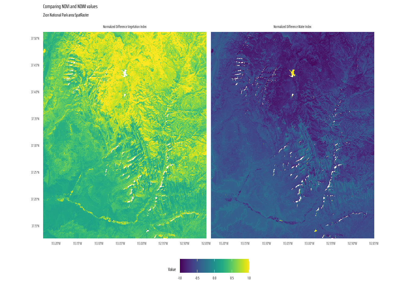
This code processes and visualizes raster data for Zion National Park, performing computations to derive vegetation and water indices and then plotting the results. The raster, containing layers for Red, Green, Blue, and Near Infrared (NIR) bands, is rescaled to real-world values, with negative values replaced by zeros.
Using custom functions, the NDVI (Normalized Difference Vegetation Index) and NDWI (Normalized Difference Water Index) are calculated from the NIR, Red, and Green bands. The resulting indices are converted into a tidy SpatRaster format for plotting.
The code below also calculates the correlation between the NDVI and NDWI layers as -0.96, thus telling us the NDVI and NDWI are negatively correlated (inversely correlated).
#################### LONG, BASE R METHOD ########################

#################### I Don't Use This ###########################

# Download the Zion National Park Raster File with layers of
# Red, Green, Blue and NIR (Near Infra Red)
landsat <- rast(
  system.file("raster/landsat.tif", package = "spDataLarge")
)

# Applying a scale factor to return values to actual ones.
# The data-set was scaled to save disk space
landsat = (landsat * 0.0000275) - 0.2

# Remove and replace negative values, since these were due to clouds
landsat[landsat < 0] = 0

# Write a custom function for computing values of
# NDVI (normalized difference vegetation index) in R
ndvi_fun = function(nir, red){
  (nir - red) / (nir + red)
}

# Create a new raster with NDVI values using terra::lapp()
landsat_ndvi <- lapp(landsat[[c(4, 3)]], fun = ndvi_fun)

# Write a custom function for computing values of
# NDWI (normalized difference water index) in R
ndwi_fun = function(nir, green){
  (green - nir) / (nir + green)
}

# Create a new raster with NDVI values using terra::lapp()
landsat_ndwi <- lapp(landsat[[c(4, 2)]], fun = ndwi_fun)

cor(
  values(landsat_ndvi),
  values(landsat_ndwi),
  use = "complete.obs"
)

# The correlation is -0.96. NDVI and NDWI are negatively correlated.
###################### THE TIDY APPROACH #######################
# Download the Zion National Park Raster File with layers of
# Red, Green, Blue and NIR (Near Infra Red)
landsat <- rast(system.file("raster/landsat.tif", package = "spDataLarge")) |>
# Applying a scale factor to return values to actual ones,
# The data-set was scaled to save disk space.
multiply_by(0.0000275) |>
subtract(0.2) |>
# Remove and replace negative values, since these were due to clouds
mutate(across(everything(), ~ ifelse(. < 0, 0, .)))
# Write a custom function for computing values of
# NDVI (normalized difference vegetation index) in R
ndvi_fun <- function(nir, red) {
(nir - red) / (nir + red)
}
# Write a custom function for computing values of
# NDWI (normalized difference water index) in R
ndwi_fun <- function(nir, green) {
(green - nir) / (green + nir)
}
# Doing the tidy data wrangling magic with tidyverse and tidyterra
landsat1 <- landsat |>
as_tibble(xy = TRUE) |>
mutate(
ndvi = ndvi_fun(landsat_4, landsat_3),
ndwi = ndwi_fun(landsat_4, landsat_2)
) |>
select(-starts_with("landsat")) |>
tidyterra::as_spatraster(
crs = st_crs(landsat)
)
# Labeller for the facets
lyr_labels <- c(
"normalized difference vegetation index",
"normalized difference water index"
) |>
str_to_title()
names(lyr_labels) <- c("ndvi", "ndwi")
layerCor(landsat1, fun = cor, use = "complete.obs") |>
round(digits = 2) [,1] [,2]
[1,] 1.00 -0.96
[2,] -0.96 1.00The ggplot2 visualization in Figure 16 uses facets to compare NDVI and NDWI values across the area, with clear labelling and a perceptually uniform colour scale.
# The actual final plot
ggplot() +
  geom_spatraster(data = landsat1) +
  scale_fill_grass_c(
    na.value = "white"
  ) +
  facet_wrap(~lyr, labeller = labeller(lyr = lyr_labels)) +
  coord_sf(expand = FALSE) +
  labs(
    title = "Comparing NDVI and NDWI values",
    subtitle = "Zion National Park area SpatRaster",
    fill = "Value"
  ) +
  theme_minimal(
    base_family = "caption_font"
  ) +
  theme(
    legend.position = "bottom",
    text = element_text(
      hjust = 0.5,
      vjust = 0.5
    )
)E8.
A StackOverflow post (stackoverflow.com/questions/35555709) shows how to compute distances to the nearest coastline using raster::distance(). Try to do something similar but with terra::distance(): retrieve a digital elevation model of Spain, and compute a raster which represents distances to the coast across the country (hint: use geodata::elevation_30s()). Convert the resulting distances from meters to kilometers. Note: it may be wise to increase the cell size of the input raster to reduce compute time during this operation (aggregate()).
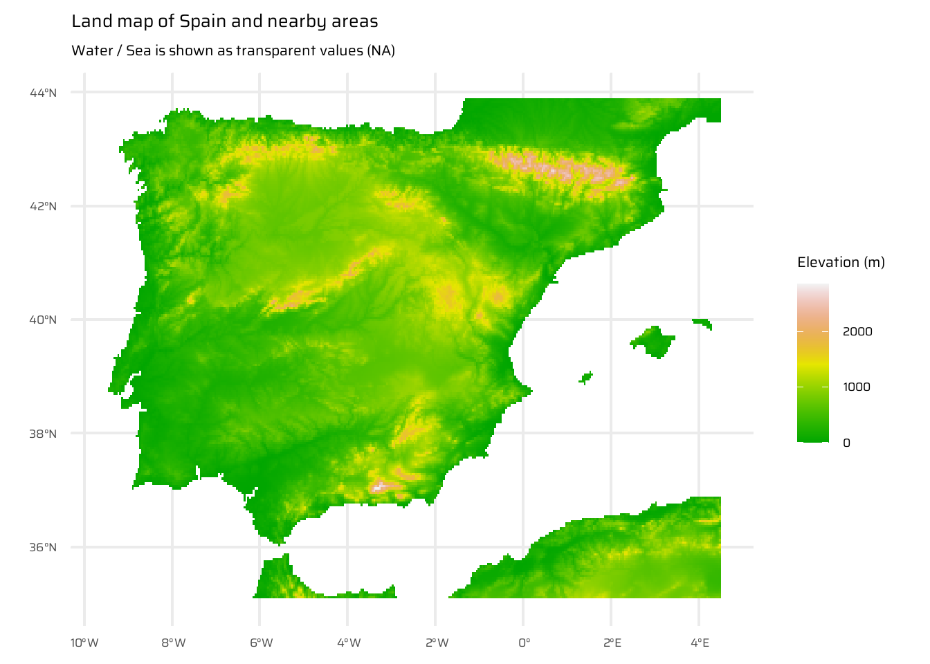
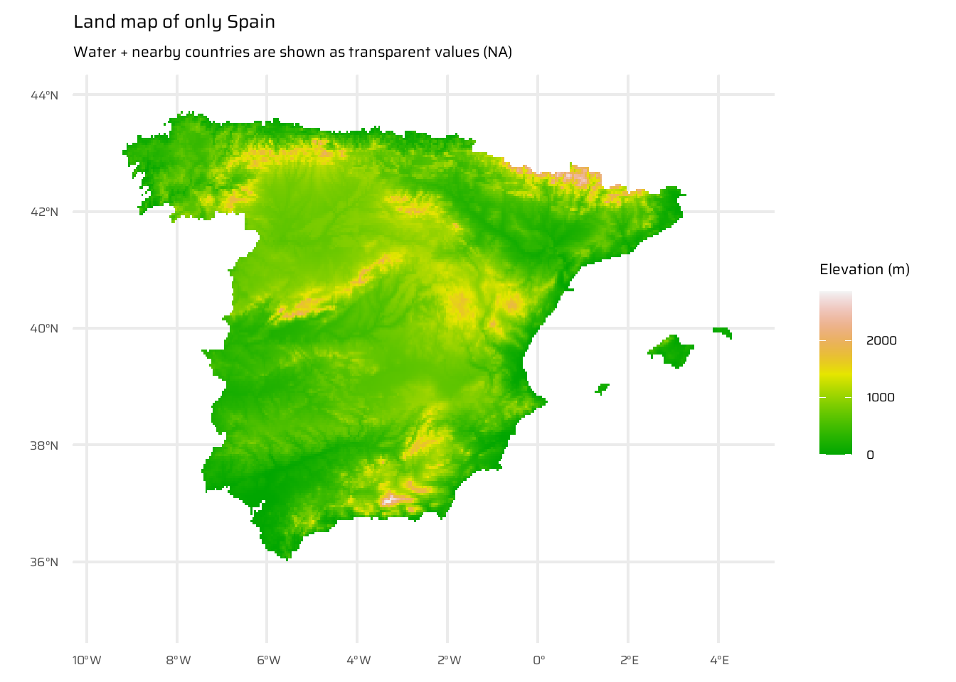
This code demonstrates the steps to compute and visualize the distance to the nearest coastline for Spain. First, it loads elevation data for Spain and nearby areas ( Figure 17 (a) ), as well as for Spain’s political boundaries ( Figure 17 (b) ), ensuring the inclusion of surrounding countries and water bodies. The raster is then aggregated for efficiency.
Initial visualizations are created: one showing elevation for Spain and neighbouring areas, and another isolating only Spain.
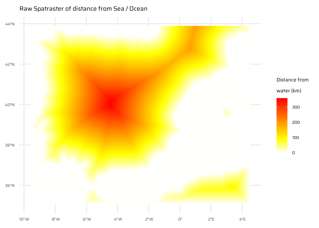
A binary raster is created where water is marked as TRUE (1) and land as NA. The distance() function calculates the distance of each land cell to the nearest water cell, with values converted to kilometres. ( Figure 17 (c) )
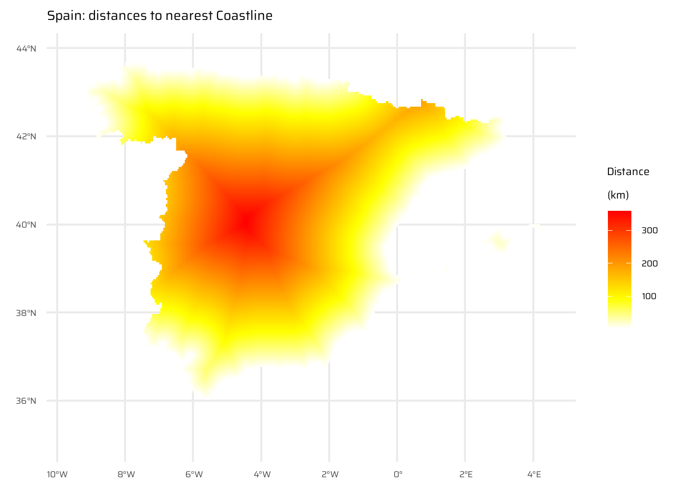
Finally, the raw distance raster is masked to display only distances within Spain, producing a final visualization of Spain with distances to its nearest coastline ( Figure 17 (d) ). The Figure 17 includes multiple stages of the process, from raw data to the final processed map.
# Full Spain and nearby Land Data
spain_land <- geodata::elevation_30s(
  country = "Spain",
  path = tempdir(),

  # Use mask = FALSE to ensure that other countries are not shown as NA
  mask = FALSE)

# Data for only Sapin Political Boundaries Land
spain_only <- geodata::elevation_30s(
  country = "Spain",
  path = tempdir()
  )

spain_working_land <- spain_land |>
  aggregate(fact = 5)

spain_working_only <- spain_only |>
  aggregate(fact = 5)

ggplot() +
  geom_spatraster(data = spain_working_land) +
  scale_fill_terrain_c(
    direction = -1
  ) +
  labs(
    title = "Land map of Spain and nearby areas",
    subtitle = "Water / Sea is shown as transparent values (NA)",
    fill = "Elevation (m)"
  )

ggplot() +
  geom_spatraster(data = spain_working_only) +
  scale_fill_terrain_c(
    direction = -1
  ) +
  labs(
    title = "Land map of only Spain",
    subtitle = "Water + nearby countries are shown as transparent values (NA)",
    fill  = "Elevation (m)"
  )

# Start with a simple raster where only water is TRUE (1)
# and land is FALSE (0)
temp <- is.na(spain_working_land)

# Convert land (i.e. FALSE) into NA
temp[temp == 0] <- NA

# Compute distance of from nearest non-NA (i.e. Water / Sea)
temp <- distance(temp)
|---------|---------|---------|---------|
=========================================
# Divide by 1000 to convert into KM
temp <- temp / 1000

ggplot() +
  geom_spatraster(data = temp) +
  paletteer::scale_fill_paletteer_c(
    "grDevices::heat.colors",
    direction = -1,
  ) +

  labs(
    fill = "Distance from\nwater (km)",
    title = "Raw Spatraster of distance from Sea / Ocean"
  )

# Convert this raw distance vector to mask and only show Spain
temp_spain <- temp |>
  # Mask it with only the map of Spain Raster
  mask(spain_working_only)

ggplot() +
  geom_spatraster(data = temp_spain) +
  paletteer::scale_fill_paletteer_c(
    "grDevices::heat.colors",
    direction = -1,
    na.value = "transparent"
  ) +
  labs(
    fill = "Distance\n(km)",
    title = "Spain: distances to nearest Coastline"
)E9.
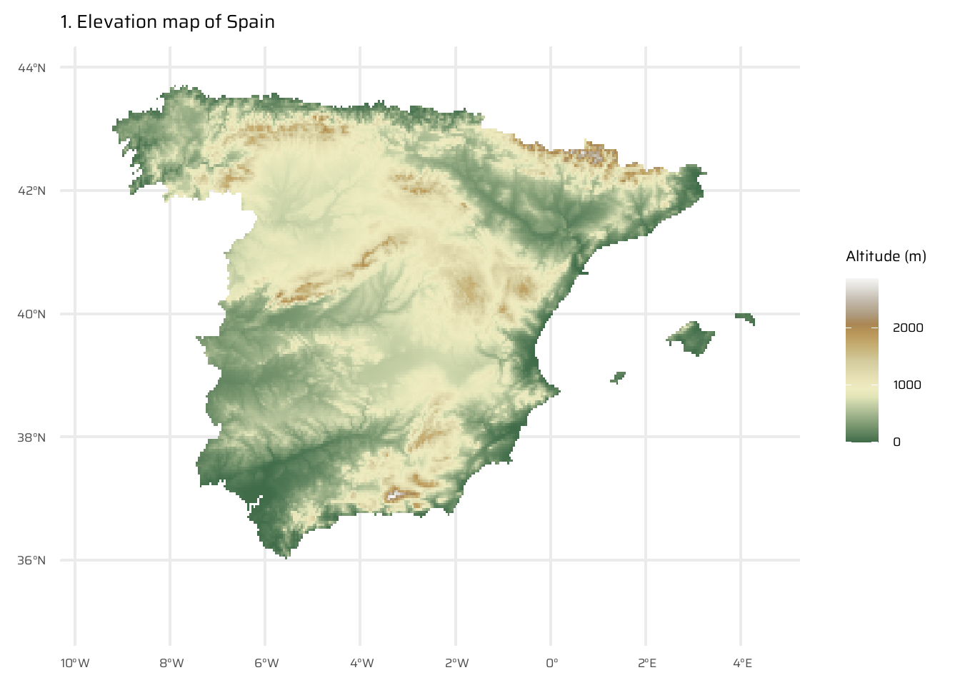
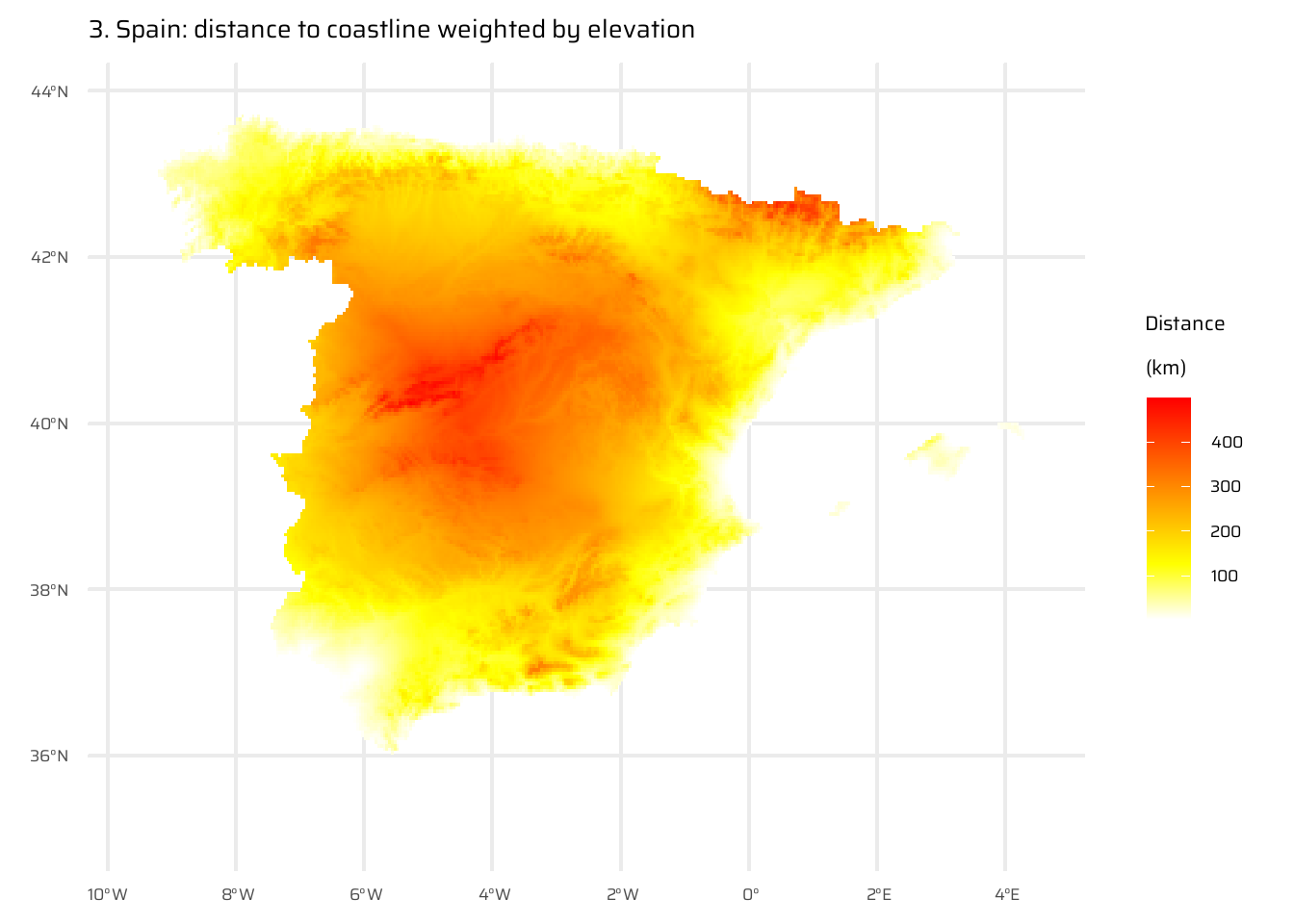
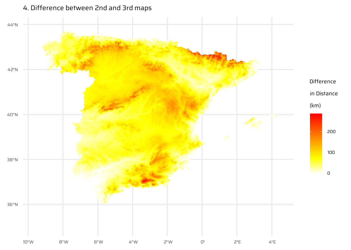
Try to modify the approach used in the above exercise by weighting the distance raster with the elevation raster; every 100 altitudinal meters should increase the distance to the coast by 10 km. Next, compute and visualize the difference between the raster created using the Euclidean distance (E7) and the raster weighted by elevation.
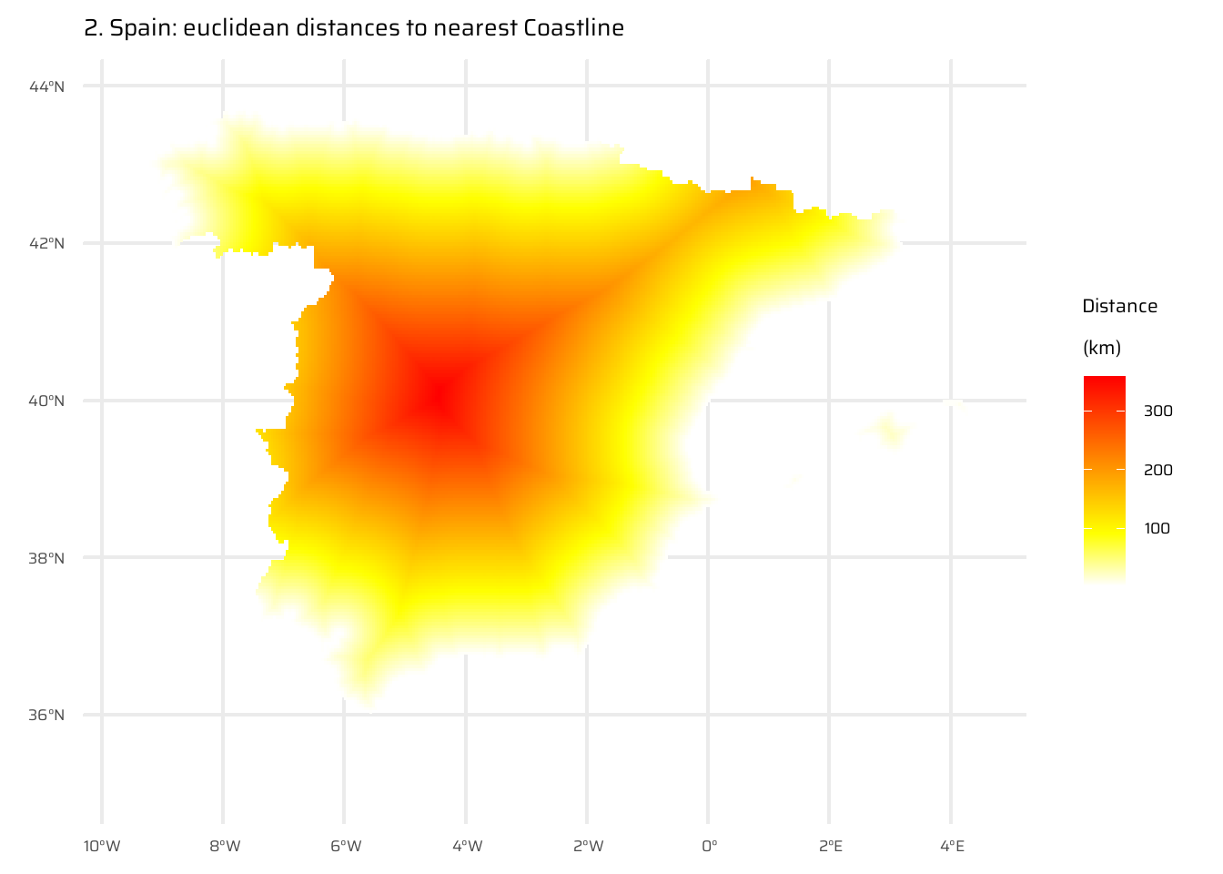
The code below performs a spatial analysis and visualization of the relationship between elevation and distance to the coastline for Spain. It begins by visualizing Spain’s elevation using a raster dataset (spain_working_only). It then calculates and visualizes the Euclidean distance from each point to the nearest coastline (temp_spain), as already done in Exercise E7.
A new raster (spain_weighted) is computed by weighting the Euclidean distance with elevation, where every 100 meters of elevation increases the effective distance to the coastline by 10 km.
The difference between the Euclidean distance raster and the elevation-weighted distance raster is then calculated and visualized (spain_difference).
The code uses the ggplot2 package to display these rasters as separate maps, with clear titles and color scales to interpret the elevation, distances, and differences.
ggplot() +
  geom_spatraster(data = spain_working_only) +
  scale_fill_wiki_c() +
  labs(
    fill = "Altitude (m)",
    title = "1. Elevation map of Spain"
  )

ggplot() +
  geom_spatraster(data = temp_spain) +
  paletteer::scale_fill_paletteer_c(
    "grDevices::heat.colors",
    direction = -1,
    na.value = "transparent"
  ) +
  labs(
    fill = "Distance\n(km)",
    title = "2. Spain: euclidean distances to nearest Coastline"
  )

spain_weighted <- temp_spain + ((spain_working_only/100) * 10)

ggplot() +
  geom_spatraster(data = spain_weighted) +
  paletteer::scale_fill_paletteer_c(
    "grDevices::heat.colors",
    direction = -1,
    na.value = "transparent"
  ) +
  labs(
    fill = "Distance\n(km)",
    title = "3. Spain: distance to coastline weighted by elevation"
  )

spain_difference <- spain_weighted - temp_spain

ggplot() +
  geom_spatraster(data = spain_difference) +
  paletteer::scale_fill_paletteer_c(
    "grDevices::heat.colors",
    direction = -1,
    na.value = "transparent"
  ) +
  labs(
    fill = "Difference\nin Distance\n(km)",
    title = "4. Difference between 2nd and 3rd maps"
  )