Creating Fishnet and Honeycomb Maps of Japan with R

Transforming prefecture boundaries into geometric grids using sf, terra, tidyterra, and ggplot2 in R

This mapping script is inspired by the insightful blog post “Beautiful Maps with R – I” by Diego Hernangómez, where he demonstrates how to craft minimalist and visually striking maps in R. Diego leverages packages such as sf for spatial data handling, terra for raster/vector operations, tidyterra for tidy‑verse–style plotting with ggplot2, and rnaturalearth for base map data. His approach blends sf::st_read() spatial workflows, terra::rast() raster processing, and mapping aesthetics via ggplot2 and tidyterra::geom_spatraster() to achieve clean, elegant results. By studying Diego’s tutorial, this code adapts and practices techniques such as layering spatial objects, customizing color palettes, and styling map themes—fully crediting Hernandez for the conceptual technique and step-by-step inspiration.

Diego Hernangómez credits his inspiration to the excellent blog post “Fishnets and Honeycomb: Square vs. Hexagonal Spatial Grids” by Matt Strimas-Mackey. In that article, Matt explores the use of alternative spatial geometries—such as square and hexagonal grids—for visualizing geographic data in more abstract or symbolic ways. His clear explanation and visual comparison of spatial tessellations sparked the idea of using simplified geometries to produce elegant map layouts. For anyone interested in innovative spatial visualization, Matt’s blog is a treasure trove of creative and technical insight.

Load packages

pacman::p_load(
  sf,          # Handling simple features objects
  terra,       # Manipulating rasters in R
  tidyterra,   # Plotting rasters with ggplot2
  
  
  tidyverse,   # Data wrangling in R
  
  
  showtext,
  ggtext,
  fontawesome,
  
  patchwork
)

Visualization Parameters

# Visualization Parameters

bts = 12 # Base Text Size
sysfonts::font_add_google("Saira Condensed", "body_font")
sysfonts::font_add_google("Saira", "title_font")
sysfonts::font_add_google("Saira Extra Condensed", "caption_font")
showtext::showtext_auto()
# A base Colour
bg_col <- "white"
seecolor::print_color(bg_col)

# Colour for highlighted text
text_hil <- "grey30"
seecolor::print_color(text_hil)

# Colour for the text
text_col <- "grey20"
seecolor::print_color(text_col)

theme_set(
  theme_minimal(
    base_size = bts,
    base_family = "body_font"
  ) +
    theme(
      text = element_text(
        colour = "grey30",
        lineheight = 0.3,
        margin = margin(0,0,0,0, "pt")
      ),
      plot.title = element_text(
        hjust = 0.5
      ),
      plot.subtitle = element_text(
        hjust = 0.5
      )
    )
)

# Caption stuff for the plot
sysfonts::font_add(
  family = "Font Awesome 6 Brands",
  regular = here::here("docs", "Font Awesome 6 Brands-Regular-400.otf")
)
github <- "&#xf09b"
github_username <- "aditya-dahiya"
xtwitter <- "&#xe61b"
xtwitter_username <- "@adityadahiyaias"
social_caption_1 <- glue::glue("<span style='font-family:\"Font Awesome 6 Brands\";'>{github};</span> <span style='color: {text_hil}'>{github_username}  </span>")
social_caption_2 <- glue::glue("<span style='font-family:\"Font Awesome 6 Brands\";'>{xtwitter};</span> <span style='color: {text_hil}'>{xtwitter_username}</span>")
plot_caption <- paste0(
  "**Data**:  {geodata}",
  "  |  **Code:** ", 
  social_caption_1, 
  " |  **Graphics:** ", 
  social_caption_2
  )
rm(github, github_username, xtwitter, 
   xtwitter_username, social_caption_1, 
   social_caption_2)

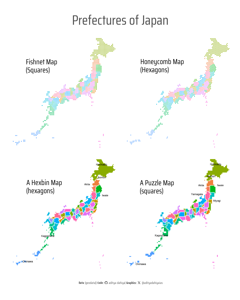
An example fishnet map for the 47 prefectures of Japan

# Download a Basic Country Map of Japan, and transform it into
# Japan Plane Rectangular CS (EPSG:30169 or Tokyo / Japan Plane Rectangular 
# CS IX) projection

base_map <- geodata::gadm(
  country = "Japan",
  level = 1,
  path = tempdir()
) |> 
  st_as_sf() |> 
  janitor::clean_names() |> 
  select(name_1,engtype_1) |> 
  st_simplify(dTolerance = 1000) |> 
  st_transform("EPSG:30169")

# base_map <- rnaturalearth::ne_countries(
#   country = "Japan",
#   returnclass = "sf",
#   scale = 50
# ) |> 
#   select(geometry) |> 
#   st_transform("EPSG:30169")

# A basic plot
# ggplot(base_map) +
#   geom_sf()

# Get hex points for the bounding box of the base map of Japan
# Then, keep only the hex points that fall within the map of Japan
# Create a grid of points covering Japan with 25km spacing
japan_points <- base_map |> 
  
  # Generate a regular grid over the extent of the base_map geometry
  st_make_grid(
    
    # Set each grid cell to be 25 kilometers (25 * 1000 meters) in size
    cellsize = 25 * 1000,     # Cell Size fo 25 km each
    
    # Use the same coordinate reference system as the base_map 
    # to ensure proper alignment
    crs = st_crs(base_map),
    
    
    # Generate center points of grid cells instead of 
    # polygons for easier point-based analysis
    what = "centers"
  ) |> 
  
  # Convert the grid points from a simple feature 
  # collection to a proper sf data frame
  st_as_sf() |> 
  
  
  # Add a unique identifier column with sequential 
  # row numbers for each grid point
  mutate(id = row_number()) |> 
  
  # Move the id column to the first position 
  # in the data frame for better visualization of tibble when inspecting
  relocate(id) |> 
  
  # Keep only the points that are within Japan
  # Perform a spatial join  - only keep those that intersect with base map
  # left = FALSE means we exclude points that don't have a match
  st_join(base_map, left = FALSE)


plot_jp_map <- function(data_japan, plot_title = ".."){
  ggplot(data_japan) +
  geom_sf(
    mapping = aes(fill = name_1),
    size = 0.2,
    colour = bg_col,
    pch = 21
  ) +
  # annotate(
  #   geom = "text",
  #   label = "Prefectures of Japan",
  #   x = 123, y = 40,
  #   size = 8,
  #   hjust = 0,
  #   family = "title_font"
  # ) +
  annotate(
    geom = "text",
    label = plot_title,
    x = 123.2, y = 39,
    size = 8,
    hjust = 0,
    family = "body_font",
    lineheight = 0.3
  ) +
  coord_sf(
    default_crs = "EPSG:4326",
    expand = FALSE
  ) + 
  ggthemes::theme_map(
    base_family = "body_font"
  ) +
  theme(
    legend.position = "none"
  )
}

g1 <- base_map |> 
  st_make_grid(
    cellsize = 40 * 1000,     # Cell Size of 40 km each
    crs = st_crs(base_map),
    what = "polygons"
  ) |> 
  st_as_sf() |> 
  mutate(id = row_number()) |> 
  relocate(id) |> 
  
  # Keep only the points that are within Japan
  st_join(base_map, left = F) |> 
  plot_jp_map(plot_title = "Fishnet Map\n(Squares)")


g2 <- base_map |> 
  st_make_grid(
    cellsize = 40 * 1000,     # Cell Size of 40 km each
    crs = st_crs(base_map),
    what = "polygons",
    square = FALSE
  ) |> 
  st_as_sf() |> 
  mutate(id = row_number()) |> 
  relocate(id) |> 
  
  # Keep only the points that are within Japan
  st_join(base_map, left = F) |> 
  plot_jp_map(plot_title = "Honeycomb Map\n(Hexagons)")

temp_df <- base_map |> 
  st_make_grid(
    cellsize = 40 * 1000,     # Cell Size of 40 km each
    crs = st_crs(base_map),
    what = "polygons",
    square = FALSE
  ) |> 
  st_as_sf() |> 
  mutate(id = row_number()) |> 
  relocate(id) |> 
  # Keep only the points that are within Japan
  st_join(base_map, left = F)
  
  
temp_df_2 <- temp_df |> 
  aggregate(
    by = list(temp_df$name_1), 
    FUN = min
  )

g3 <- temp_df_2 |> 
  plot_jp_map(plot_title = "A Hexbin Map\n(hexagons)")  +
  ggrepel::geom_text_repel(
    data = temp_df_2,
    mapping = aes(label = name_1, geometry = geometry),
    size = 3,
    stat = "sf_coordinates",
    force = 0.5,
    force_pull = 10,
    max.overlaps = 10,
    min.segment.length = unit(100, 'pt')
  )


temp_df <- base_map |> 
  st_make_grid(
    cellsize = 40 * 1000,     # Cell Size of 40 km each
    crs = st_crs(base_map),
    what = "polygons"
  ) |> 
  st_as_sf() |> 
  mutate(id = row_number()) |> 
  relocate(id) |> 
  # Keep only the points that are within Japan
  st_join(base_map, left = F)
  
temp_df_2 <- temp_df |> 
  aggregate(
    by = list(temp_df$name_1), 
    FUN = min
  )
  
g4 <- temp_df_2 |> 
  plot_jp_map(plot_title = "A Puzzle Map\n(squares)") +
  ggrepel::geom_text_repel(
    data = temp_df_2,
    mapping = aes(label = name_1, geometry = geometry),
    size = 3,
    stat = "sf_coordinates",
    force = 0.5,
    force_pull = 10,
    max.overlaps = 10,
    min.segment.length = unit(100, 'pt')
  )

library(patchwork)

g <- g1 + g2 + g3 + g4 +
  plot_annotation(
    title = "Prefectures of Japan",
    caption = plot_caption,
    theme = theme(
      plot.title = element_text(
        size = 42
      ),
      plot.caption = element_textbox(
        hjust = 0.5
      )
    )
  )

Saving the map

size_var = 1000

ggsave(
  plot = g,
  filename = here::here(
    "geocomputation", 
    "images",
    "fishnet_maps_1.png"
  ),
  width = size_var,
  height = (5/4) * size_var,
  units = "px",
  bg = bg_col
)

Figure 1: Four visualization approaches to transform Japan’s administrative boundaries into abstract geometric patterns. The fishnet map (top left) uses regular square grids, while the honeycomb map (top right) employs hexagonal tessellations for smoother visual flow. The hexbin and puzzle maps (bottom panels) aggregate these geometric shapes by prefecture, creating simplified representations where each administrative unit is depicted as a single polygon with labeled centroids, offering cleaner cartographic alternatives to traditional boundary maps.

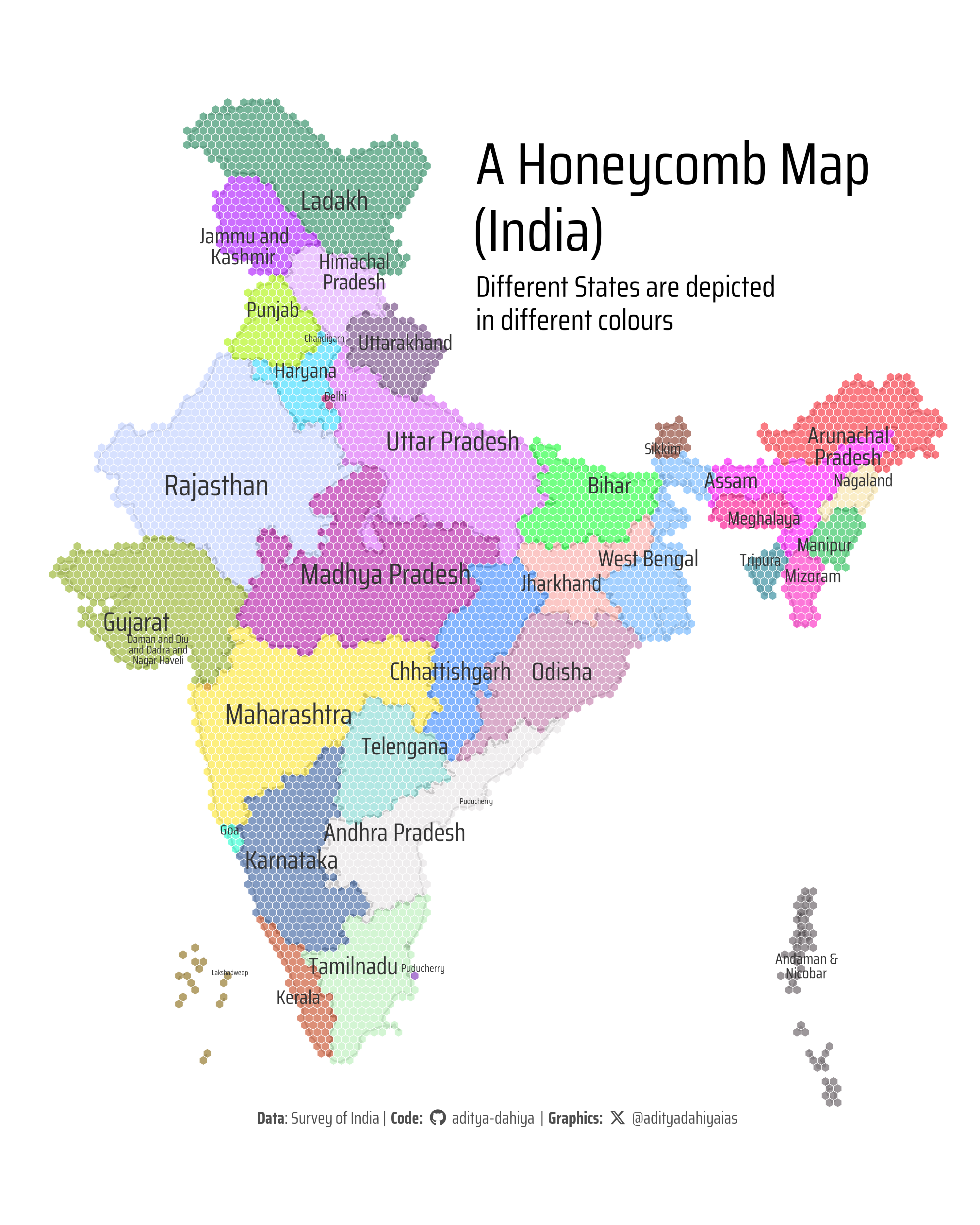
An example for Map of India and its states

This R script creates a visually striking “honeycomb map” of India by overlaying a hexagonal grid pattern on the country’s state boundaries. The code primarily leverages the powerful {sf} (Simple Features) package for spatial data manipulation and geometric operations, including reading shapefiles with read_sf(), creating hexagonal grids with st_make_grid(), and performing spatial joins with st_join(). The visualization is built using {ggplot2} with its spatial extension geom_sf() for mapping, while {ggrepel} handles intelligent label positioning to avoid overlaps. Additional functionality comes from {paletteer} for accessing a diverse color palette, {janitor} for data cleaning with clean_names(), and {here} for robust file path management. The result is an aesthetically pleasing cartographic representation where each hexagonal cell is colored according to the Indian state it overlaps with most, creating a unique geometric interpretation of India’s political geography.

india <- read_sf(
  here::here(
    "data",
    "india_map",
    "India_State_Boundary.shp"
  )
) |> 
  janitor::clean_names()

object.size(india) |> print(units = "Kb")

st_crs(india)

mypal <- paletteer::paletteer_d("Polychrome::palette36")

# Create a grid of points covering Japan with 25km spacing
india_fishnet <- india |> 
  
  # Simplyfy the geometry to make processing quick and avoid slivers
  st_simplify(dTolerance = 10000) |> 
  
  # Generate a regular grid over the extent of the base_map geometry
  st_make_grid(
    
    # Set each grid cell to be specified kilometers (... * 1000 meters) in size
    cellsize = 30 * 1000,     # Cell Size 
    
    # Use the same coordinate reference system as the base_map 
    # to ensure proper alignment
    crs = st_crs(india),
    
    
    # Generate center points of grid cells instead of 
    # polygons for easier point-based analysis
    what = "polygons",
    
    # Whether to make it square or hex
    square = FALSE
  ) |> 
  
  # Convert the grid points from a simple feature 
  # collection to a proper sf data frame
  st_as_sf() |> 
  
  
  # Add a unique identifier column with sequential 
  # row numbers for each grid point
  mutate(id = row_number()) |> 
  
  # Move the id column to the first position 
  # in the data frame for better visualization of tibble when inspecting
  relocate(id) |> 
  
  # Keep only the points that are within Japan
  # Perform a spatial join  - only keep those that intersect with base map
  # left = FALSE means we exclude points that don't have a match
  st_join(
    india,
    
    # Only return the state that has the largest overlap with a hexagon
    largest = TRUE,
    
    # To perform a left join, i.e. retain the hexagons that intersect with
    # each state
    left = FALSE
  )


######
# Caption stuff for the plot
sysfonts::font_add(
  family = "Font Awesome 6 Brands",
  regular = here::here("docs", "Font Awesome 6 Brands-Regular-400.otf")
)
github <- "&#xf09b"
github_username <- "aditya-dahiya"
xtwitter <- "&#xe61b"
xtwitter_username <- "@adityadahiyaias"
social_caption_1 <- glue::glue("<span style='font-family:\"Font Awesome 6 Brands\";'>{github};</span> <span style='color: {text_hil}'>{github_username}  </span>")
social_caption_2 <- glue::glue("<span style='font-family:\"Font Awesome 6 Brands\";'>{xtwitter};</span> <span style='color: {text_hil}'>{xtwitter_username}</span>")
plot_caption <- paste0(
  "**Data**:  Survey of India",
  "  |  **Code:** ", 
  social_caption_1, 
  " |  **Graphics:** ", 
  social_caption_2
  )
rm(github, github_username, xtwitter, 
   xtwitter_username, social_caption_1, 
   social_caption_2)

######
g <- india_fishnet |> 
  ggplot() +
  geom_sf(
    data = india,
    linewidth = 0.6,
    alpha = 0.2, 
    fill = NA,
    colour = alpha("black", 0.2)
  ) +
  geom_sf(
    mapping = aes(
      fill = state_name
    ),
    colour = bg_col,
    linewidth = 0.2,
    alpha = 0.6
  ) +
  ggrepel::geom_text_repel(
    data = india |> mutate(state_area = as.numeric(st_area(geometry))),
    mapping = aes(
      label = str_wrap(state_name, 15),
      geometry = geometry,
      size = state_area
    ),
    stat = "sf_coordinates",
    box.padding = 0.1,
    min.segment.length = unit(100, "pt"),
    family = "body_font",
    seed = 42,
    colour = text_col,
    lineheight = 0.25
  ) +
  
  annotate(
    geom = "text",
    x = 82,
    y = 33,
    label = "A Honeycomb Map\n(India)",
    size = 4 * bts,
    hjust = 0, vjust = 0,
    family = "body_font",
    lineheight = 0.3
  ) +
  annotate(
    geom = "text",
    x = 82,
    y = 32.3,
    label = "Different States are depicted\nin different colours",
    size = 2 * bts,
    hjust = 0, vjust = 1,
    family = "body_font",
    lineheight = 0.3
  ) +
  coord_sf(
    expand = FALSE,
    default_crs = "EPSG:4326"
  ) +
  scale_fill_manual(
    values = mypal
  ) +
  scale_colour_manual(
    values = mypal
  ) +
  scale_size_continuous(range = c(bts / 2, bts * 2), trans = "sqrt") +
  labs(caption = plot_caption) +
  ggthemes::theme_map(
    base_family = "body_font",
    base_size = bts * 4
  ) +
  theme(
    legend.position = "none",
    plot.caption = element_textbox(
      hjust = 0.5, 
      margin = margin(-10,0,0,0, "pt"),
      colour = text_hil
    )
  )

size_var = 3000

ggsave(
  plot = g,
  filename = here::here(
    "geocomputation", 
    "images",
    "fishnet_maps_2.png"
  ),
  width = size_var,
  height = (5/4) * size_var,
  units = "px",
  bg = bg_col
)

Figure 2: A Honeycomb View of India: This geometric representation transforms India’s political map into a striking hexagonal mosaic. Each coloured hexagon corresponds to the state or union territory it overlaps with most, creating a stylized yet geographically recognizable portrayal of the subcontinent. The different colors reveal India’s 28 states and 8 union territories offering a fresh perspective on the country’s diverse political landscape.