Cropping {ggmap} rasters with {terra} to make beautiful maps

Combining the feautres of {ggmap}, {osmdata}, {terra} and {tidyterra}

Loading Libraries

# Data wrangling & visualization
library(tidyverse)  # Data manipulation & visualization

# Spatial data handling
library(sf)         # Import, export, and manipulate vector data
library(terra)      # Import, export, and manipulate raster data

# ggplot2 extensions
library(tidyterra)  # Helper functions for using terra with ggplot2

# Getting raster tiles
library(ggmap)      # Getting map raster tiles
library(osmdata)    # Get Open Street Maps

# Final plot tools
library(scales)               # Nice Scales for ggplot2
library(fontawesome)          # Icons display in ggplot2
library(ggtext)               # Markdown text in ggplot2
library(showtext)             # Display fonts in ggplot2
library(patchwork)            # Composing Plots

bts = 12 # Base Text Size
sysfonts::font_add_google("Roboto Condensed", "body_font")
sysfonts::font_add_google("Oswald", "title_font")
sysfonts::font_add_google("Saira Extra Condensed", "caption_font")

showtext::showtext_auto()
# A base Colour
bg_col <- "white"
seecolor::print_color(bg_col)

# Colour for highlighted text
text_hil <- "grey30"
seecolor::print_color(text_hil)

# Colour for the text
text_col <- "grey20"
seecolor::print_color(text_col)

theme_set(
  theme_minimal(
    base_size = bts,
    base_family = "body_font"
  ) +
    theme(
      text = element_text(
        colour = "grey30",
        lineheight = 0.3,
        margin = margin(0,0,0,0, "pt")
      ),
      plot.title = element_text(
        hjust = 0.5
      ),
      plot.subtitle = element_text(
        hjust = 0.5
      )
    )
)

# Caption stuff for the plot
sysfonts::font_add(
  family = "Font Awesome 6 Brands",
  regular = here::here("docs", "Font Awesome 6 Brands-Regular-400.otf")
)
github <- "&#xf09b"
github_username <- "aditya-dahiya"
xtwitter <- "&#xe61b"
xtwitter_username <- "@adityadahiyaias"
social_caption_1 <- glue::glue("<span style='font-family:\"Font Awesome 6 Brands\";'>{github};</span> <span style='color: {text_hil}'>{github_username}  </span>")
social_caption_2 <- glue::glue("<span style='font-family:\"Font Awesome 6 Brands\";'>{xtwitter};</span> <span style='color: {text_hil}'>{xtwitter_username}</span>")
plot_caption <- paste0(
  "**Data**:  StadiaMaps & Open Street Maps",
  "  |  **Code:** ", 
  social_caption_1, 
  " |  **Graphics:** ", 
  social_caption_2
  )
rm(github, github_username, xtwitter, 
   xtwitter_username, social_caption_1, 
   social_caption_2)

Getting, cropping, masking and plotting raster maps

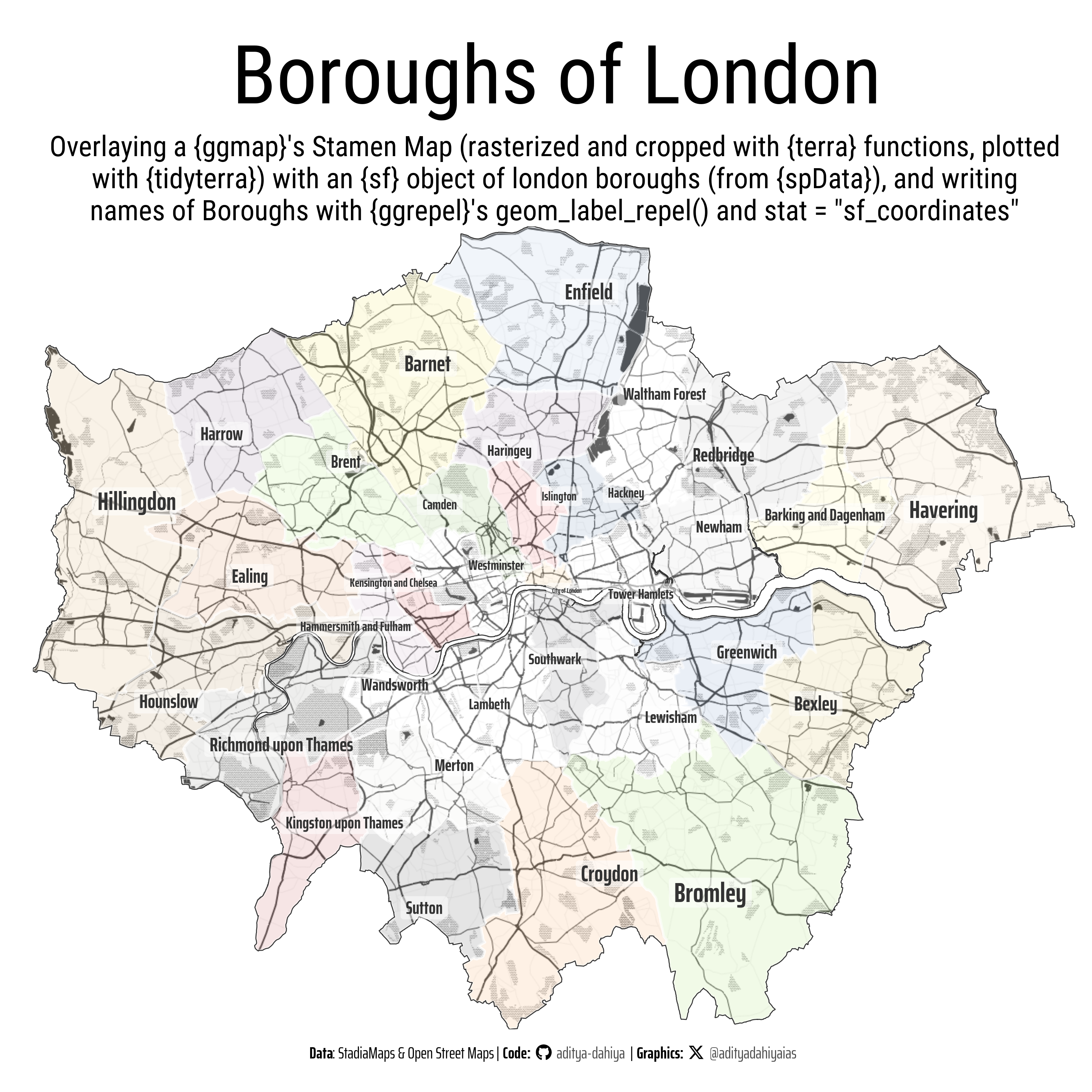
This code leverages multiple R packages to create a detailed map of London Boroughs, integrating rasterized map tiles with spatial vector data. The {sf} package is used to obtain and manipulate the bounding box of London Boroughs, while {spData} provides the spatial dataset. The {ggmap} package is used to fetch base map tiles from Stamen Maps via get_stadiamap(), and {terra} functions like rast(), crop(), and mask() are applied to process and refine these tiles. The map visualization is built using {ggplot2}, with additional enhancements from {ggrepel} for labeling borough names, {paletteer} for colour scaling, and {ggthemes} for theming. The final visualization overlays London Boroughs on the map tiles, applying transparency and borders for clarity, and saves the output using {here}.

# Obtain the bounding box of London Boroughs
london_bbox <- sf::st_bbox(spData::lnd)

# A bounding box in the format c(lowerleftlon, lowerleftlat, upperrightlon, upperrightlat)
london_bbox <- c(
  left = london_bbox$xmin,
  right = london_bbox$xmax,
  bottom = london_bbox$ymin,
  top = london_bbox$ymax
)
names(london_bbox) <- c("left", "right", "bottom", "top")

# Getting London Boroughs Data
df <- spData::lnd |>
  st_transform("EPSG:4326")

# Register stadia maps API key
# register_stadiamaps("Your-Key-Here")

# Getting the map tiles
# london_base1 <- get_stadiamap(
#   bbox = london_bbox,
#   zoom = 11,
#   maptype = "stamen_toner_lines"
# )

london_base2 <- get_stadiamap(
  bbox = london_bbox,
  zoom = 11,
  maptype = "stamen_toner_background"
)

# Convert {ggmap} object into a SpatRaster
london_base3 <- london_base2 |> 
  rast() |> 
  crop(df) |> 
  mask(df)

# Starting with base map tiles
g <- ggplot() +
  
  # Plotting the cropped raster map
  geom_spatraster_rgb(
    data = london_base3,
    maxcell = Inf,
    alpha = 0.7
  ) +
  
  # Plotting the London boroughs
  geom_sf(
    data = df,
    aes(fill = NAME),
    alpha = 0.1,
    linewidth = 0.8,
    colour = alpha("white", 0.5)
  ) +
  paletteer::scale_fill_paletteer_d("palettesForR::Tango") +
  
  # Plotting overall border of London City
  geom_sf(
    data = df |> st_geometry() |> st_union(),
    colour = text_col,
    linewidth = 0.3,
    fill = NA
  ) +
  
  # Plotting names of London Boroughs on top of the geom_sf
  ggrepel::geom_label_repel(
    data = df,
    aes(label = NAME, geometry = geometry, size = HECTARES),
    fill = alpha("white", 0.5),
    colour = text_col,
    family = "caption_font",
    fontface = "bold",
    label.size = unit(0, "pt"),
    stat = "sf_coordinates"
  ) +
  scale_size_continuous(range = c(5, 20)) +
  
  coord_sf(expand = FALSE) +
  
  # Labels
  labs(
    title = "Boroughs of London",
    subtitle = str_wrap("Overlaying a {ggmap}'s Stamen Map (rasterized and cropped with {terra} functions, plotted with {tidyterra}) with an {sf} object of london boroughs (from {spData}), and writing names of Boroughs with {ggrepel}'s geom_label_repel() and stat = \"sf_coordinates\"", 90),
    caption = plot_caption
  ) +
  
  # Some theme elements
  ggthemes::theme_map(
    base_size = bts,
    base_family = "body_font"
  ) +
  theme(
    legend.position = "none",
    plot.title = element_text(
      size = 4 * bts,
      margin = margin(30,0,10,0, "pt"),
      hjust = 0.5
    ),
    plot.subtitle = element_text(
      margin = margin(0,0,0,0, "pt"),
      lineheight = 0.3,
      size = bts * 1.4,
      hjust = 0.5
    ),
    plot.caption = element_textbox(
      margin = margin(0,0,20,0, "pt"),
      hjust = 0.5,
      halign = 0.5,
      family = "caption_font"
    ),
    plot.margin = margin(0,-10,0,-10, "pt")
  )

ggsave(
  filename = here::here("geocomputation", 
                        "images", 
                        "ggmap_terra_1.png"),
  plot = g,
  height = 3000,
  width = 3000,
  units = "px",
  bg = "white"
)

Figure 1: A raster tile maps of Stamen Toner Background for London area, plotted at the base. London Boroughs’ borders plotted on top of it, along with names of the boroughs.

# haryana <- geodata::gadm(
#   country = "India",
#   level = 3,
#   path = tempdir()
# )
# 
# haryana |> 
#   janitor::clean_names() |> 
#   filter(name_1 == "Haryana") |> 
#   st_as_sf() |> 
#   ggplot() +
#   geom_sf() +
#   geom_sf_text(
#     size = 3,
#     mapping = aes(label = name_3)
#   )

haryana <- read_sf(
  here::here(
    "data", "haryana_map",
    "HARYANA_SUBDISTRICT_BDY.shp"
  )
) |> 
  janitor::clean_names() |> 
  mutate(
    district = str_replace_all(district, ">", "A"),
    district = str_replace_all(district, "\\|", "I"),
    district = str_to_title(district),
    tehsil = str_replace_all(tehsil, ">", "A"),
    tehsil = str_replace_all(tehsil, "\\|", "I"),
    tehsil = str_to_title(tehsil)
  ) |> 
  st_simplify(dTolerance = 100) |> 
  select(-state, -shape_leng, -shape_area)

haryana_boundary

haryana |> 
  st_union() |> 
  st_cast("POLYGON") |> 
  st_as_sf() |> 
  slice(1) |> 
  ggplot() +
  geom_sf()

  
ggplot() +
  geom_sf(data = haryana_boundary)

Mapping a Coastal Town - Vladivostok

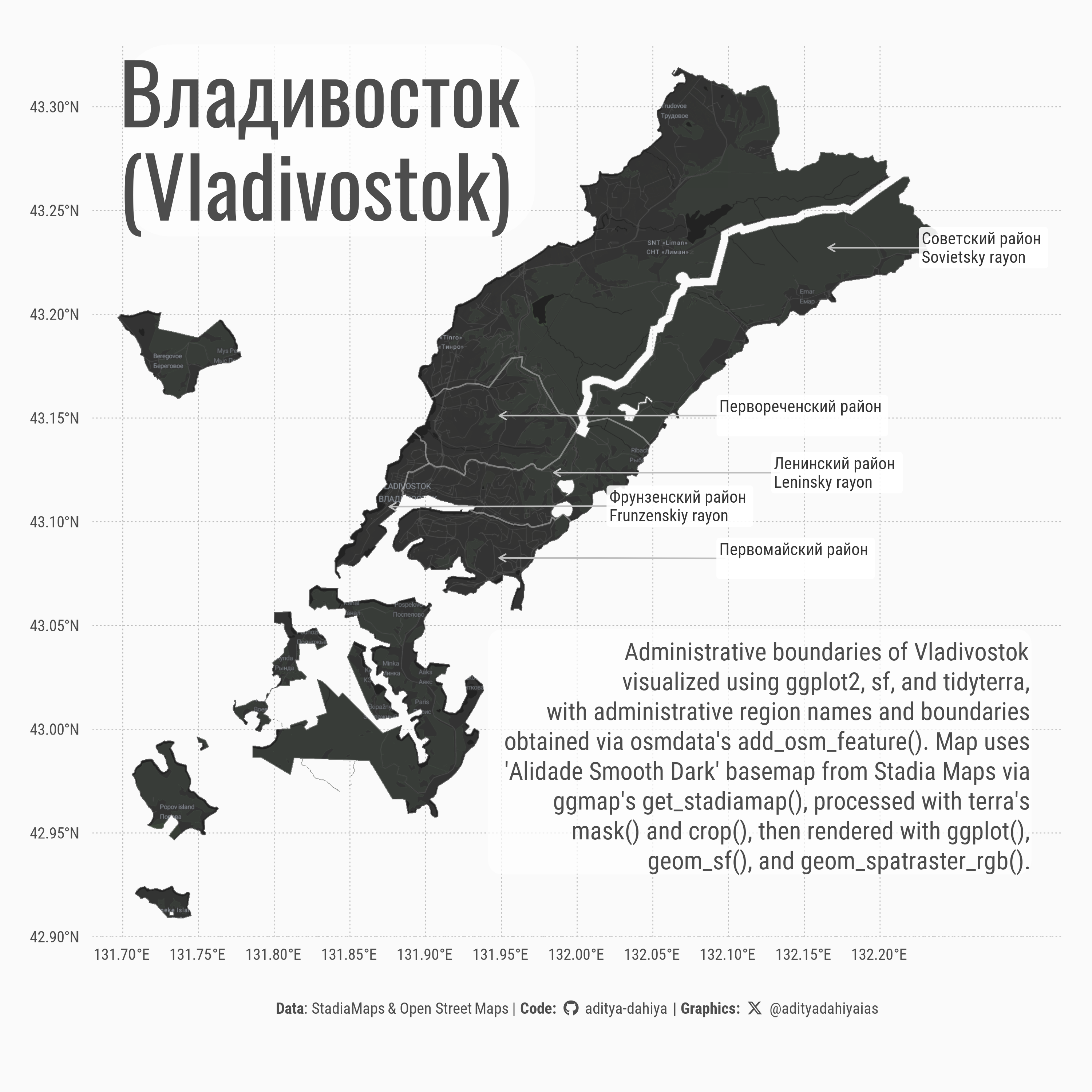
This code showcases the creation of a detailed administrative map of Vladivostok using a powerful combination of R spatial packages. The workflow begins by retrieving administrative boundary data via the osmdata package, then processes these geometries using sf for spatial operations. The map incorporates a stylish dark basemap from Stadia Maps, accessed through ggmap, which is then carefully cropped and masked to the city boundaries using terra functions. The visualization layer, built with ggplot2, combines the raster basemap with vector boundaries and elegantly positioned labels using ggrepel. The code demonstrates a sophisticated integration of multiple spatial data processing techniques—from acquisition to transformation to visualization—resulting in a professional-quality map that highlights Vladivostok’s administrative regions with both Russian and English labels. The approach illustrates modern R spatial data visualization practices, combining the strengths of multiple packages to handle different aspects of the geospatial workflow.

Inspiration Code for custom CRS projections, written by me for another page. May Style Library (for the StadiaMaps)

# Background Colour
bg_col <- "white"
city_bb <- osmdata::getbb("Vladivostok")

city_map <- opq(bbox = city_bb) |> 
  add_osm_feature(
    key = "boundary",
    value = "administrative"
  ) |> 
  osmdata_sf()

new_crs <- paste0(
  "+proj=laea +x_0=0 +y_0=0 +lon_0=", mean(city_bb[1, 1], city_bb[1, 2]), 
  " +lat_0=", mean(city_bb[2, 1], city_bb[2, 2])
)

# register_stadiamaps("your-key-here")
# Convert bbox to a polygon
coords <- matrix(c(
  city_bb["x", "min"], city_bb["y", "min"],  # bottom-left
  city_bb["x", "max"], city_bb["y", "min"],  # bottom-right
  city_bb["x", "max"], city_bb["y", "max"],  # top-right
  city_bb["x", "min"], city_bb["y", "max"],  # top-left
  city_bb["x", "min"], city_bb["y", "min"]   # back to start to close polygon
), ncol = 2, byrow = TRUE)

# Create sf polygon object
city_poly <- st_polygon(list(coords)) %>%
  st_sfc() |>                     # create simple feature collection
  st_sf() |>                      # convert to sf object
  st_set_crs("EPSG:4326")
rm(coords)

city_map1 <- city_map$osm_multipolygons |>
  select(osm_id, name, admin_level, geometry, `name:en`, name) |> 
  filter(admin_level == 9)

city_border <- city_map1 |> 
  st_geometry() |> 
  st_union()

stadia_bbox <- st_bbox(city_border)
names(stadia_bbox) <- c("left", "bottom", "right", "top")

raw_rast <- get_stadiamap(
  bbox = stadia_bbox,
  zoom = 12,
  maptype = "alidade_smooth_dark"
)

rast <- raw_rast |> 
  terra::rast() |> 
  terra::crop(city_map1) |>
  terra::mask(city_map1, touches = FALSE)

city_map$osm_multipolygons |> 
  st_drop_geometry() |> 
  as_tibble() |> 
  select(`name:en`, name, osm_id)

city_names <- city_map$osm_multipolygons |> 
  st_centroid() |> 
  select(name, `name:en`) |> 
  st_crop(city_poly)

g <- ggplot() +
  geom_spatraster_rgb(
    data = rast,
    maxcell = 1e8
  ) +
  geom_sf(
    data = city_map1,
    fill = NA,
    colour = alpha("white", 0.2),
    linewidth = 0.5
  ) +
  ggrepel::geom_label_repel(
    data = city_map1,
    mapping = aes(
      label = paste0(name, "\n",`name:en`),
      geometry = geometry
    ),
    family = "body_font",
    lineheight = 0.3,
    fill = alpha("white", 0.9),
    stat = "sf_coordinates",
    colour = "grey20",
    size = 12,
    hjust = 0,
    label.size = NA,
    nudge_x = 0.15,
    direction = "y",
    arrow = arrow(
      length = unit(5, "pt")
    ), 
    segment.colour = "grey"
  ) +
  annotate(
    geom = "label",
    x = 131.7,
    y = 43.33,
    label = "Владивосток\n(Vladivostok)",
    family = "title_font",
    size = 60,
    hjust = 0,
    vjust = 1,
    lineheight = 0.3,
    colour = text_hil,
    fill = alpha(bg_col, 0.7),
    label.padding = unit(0.02, "lines"),
    label.size = NA
  ) +
  annotate(
    geom = "label",
    x = 132.3,
    y = 42.93,
    label = str_wrap("Administrative boundaries of Vladivostok visualized using ggplot2, sf, and tidyterra, with administrative region names and boundaries obtained via osmdata's add_osm_feature(). Map uses 'Alidade Smooth Dark' basemap from Stadia Maps via ggmap's get_stadiamap(), processed with terra's mask() and crop(), then rendered with ggplot(), geom_sf(), and geom_spatraster_rgb().", 50),
    family = "body_font",
    size = 18,
    hjust = 1,
    vjust = 0,
    lineheight = 0.32,
    fill = alpha(bg_col, 0.7),
    label.padding = unit(0.1, "lines"),
    label.size = NA,
    colour = text_hil
  ) +
  labs(
    x = NULL, y = NULL,
    caption = plot_caption
  ) +
  scale_x_continuous(
    limits = c(131.68, 132.32),
    breaks = seq(131.7, 132.2, 0.05)
  ) +
  scale_y_continuous(
    limits = c(42.9, 43.33),
    breaks = seq(42.9, 43.3, 0.05)
  ) +
  coord_sf(
    expand = FALSE,
    default_crs = "EPSG:4326"
  ) +
  theme_minimal(
    base_size = 40,
    base_family = "body_font"
  ) +
  theme(
    panel.grid = element_line(
      linewidth = 0.3,
      linetype = 3,
      colour = "grey"
    ),
    axis.ticks = element_blank(),
    axis.ticks.length = unit(0, "pt"),
    plot.caption = element_textbox(
      hjust = 0.5,
      halign = 0.5,
      margin = margin(25,0,20,0, "pt"),
      colour = text_hil
    )
  )

ggsave(
  filename = here::here("geocomputation", 
                        "images", 
                        "ggmap_terra_2.png"),
  plot = g,
  height = 3000,
  width = 3000,
  units = "px",
  bg = "grey98"
)

Figure 2: This visualization highlights the administrative districts of Vladivostok, Russia, with both Russian and English labels to enhance accessibility. The dark basemap creates a striking contrast with the white boundary lines, emphasizing the city’s complex geography where land meets the Sea of Japan. Each district is clearly delineated, revealing how Vladivostok’s urban structure has been shaped by its mountainous peninsula location and its historical importance as Russia’s major Pacific port.

Stylized Maps with {ggmap} and {osmdata}

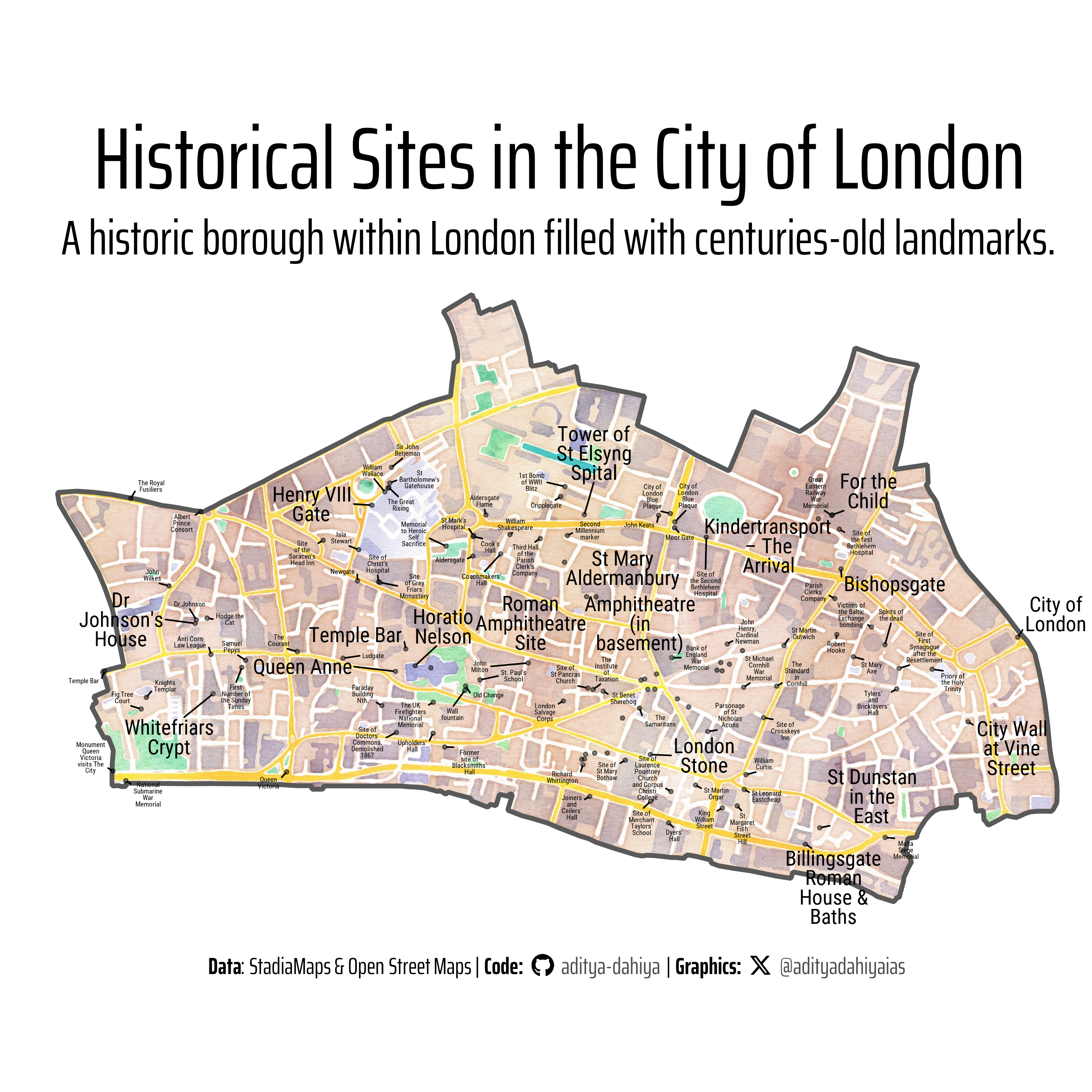
This code extracts the boundary of the City of London from the spData package and processes it using sf functions. It defines a bounding box for the area and retrieves a watercolor-style basemap from get_stadiamap(). Using osmdata, historical sites within the City of London—such as castles, memorials, and ruins—are queried from OpenStreetMap. The extracted data is filtered, transformed, and plotted with ggplot2, overlaying the historical landmarks on the base map. Labels are added using ggrepel to improve readability. The final visualization is saved using ggsave().

city_of_london <- spData::lnd |> 
  janitor::clean_names() |> 
  filter(name == "City of London") |> 
  st_transform("EPSG:4326")

# Obtain the bounding box of London Boroughs
london_bbox <- sf::st_bbox(city_of_london)
london_bbox2 <- sf::st_bbox(city_of_london)

# A bounding box in the format c(lowerleftlon, lowerleftlat, upperrightlon, upperrightlat)
london_bbox <- c(
  left = london_bbox$xmin,
  right = london_bbox$xmax,
  bottom = london_bbox$ymin,
  top = london_bbox$ymax
)
names(london_bbox) <- c("left", "right", "bottom", "top")

# Register stadia maps API key
# register_stadiamaps("Your-Key-Here")

london_city_base <- get_stadiamap(
  bbox = london_bbox,
  zoom = 16,
  maptype = "stamen_watercolor"
)

base1 <- rast(london_city_base) |> 
  crop(city_of_london) |> 
  mask(city_of_london, touches = FALSE)

df1 <- osmdata::opq(bbox = london_bbox2) |> 
  osmdata::add_osm_feature(
    key = "historic",
    value = c("archaeological_site", "battlefield", "boundary_stone", "building", "castle", "city_gate", "citywalls", "fort", "manor", "memorial", "milestone", "monument", "ruins", "ship", "tomb", "wayside_cross", "wayside_shrine")

  ) |> 
  osmdata_sf()


df2 <- bind_rows(
  # df1$osm_multipolygons |> 
  #   filter(!is.na(name)) |> 
  #   select(name),
  
  df1$osm_polygons |> 
    filter(!is.na(name)) |> 
    select(name, historic) |> 
    st_centroid(),

  df1$osm_points |> 
    filter(!is.na(name)) |> 
    select(name, historic),
) |>
  st_transform("EPSG:4326") |> 
  st_intersection(city_of_london) |> 
  select(name, historic) |> 
  mutate(size_var = if_else(historic == "memorial", 5, 15))

df2 |> 
  st_drop_geometry() |> 
  as_tibble() |> 
  count(historic)

g <- ggplot() +
  geom_spatraster_rgb(
    data = base1,
    maxcell = Inf,
    alpha = 0.75
  ) +
  geom_sf(
    data = city_of_london,
    fill = NA,
    linewidth = 1.5,
    alpha = 0.5,
    linejoin = "bevel"
  ) +
  geom_sf(
    data = df2,
    fill =  NA,
    alpha = 0.5,
    size = 1
  ) +
  ggrepel::geom_text_repel(
    data = df2,
    mapping = aes(
      label = str_wrap(name, 10, whitespace_only = F),
      geometry = geometry,
      size = size_var
    ),
    lineheight = 0.25,
    family = "body_font",
    stat = "sf_coordinates",
    min.segment.length = unit(0, "pt"),
    force = 1,
    force_pull = 0.5,
    seed = 42,
    linewidth = 0.1
  ) +
  scale_size_identity() +
  labs(
    x = NULL, y = NULL,
    caption = plot_caption,
    title = "Historical Sites in the City of London",
    subtitle = "A historic borough within London filled with centuries-old landmarks."
  ) +
  ggthemes::theme_map(
    base_family = "body_font",
    base_size = 60
  ) +
  theme(
    plot.caption = element_textbox(
      hjust = 0.5,
      halign = 0.5,
      family = "caption_font",
      margin = margin(0,0,0,0, "pt")
    ),
    plot.title = element_text(
      margin = margin(10,0,5,0, "pt"),
      size = 180,
      family = "caption_font",
      hjust = 0.5
    ),
    plot.subtitle = element_text(
      margin = margin(5,0,0,0, "pt"),
      size = 100,
      hjust = 0.5,
      family = "caption_font"
    ),
    plot.margin = margin(0,-10,0,-10, "pt")
  )
 

ggsave(
  filename = here::here("geocomputation", 
                        "images", 
                        "ggmap_terra_3.png"),
  plot = g,
  height = 3000,
  width = 3000,
  units = "px",
  bg = "white"
)

Figure 3: Map of historical sites in the City of London, overlaid on a watercolor-style basemap. The visualization highlights key landmarks such as castles, monuments, and memorials, with point sizes indicating their type and significance.