Showing elevation in Maps (1) : {hillshader}

Exploring {hillshader} for shaded relief maps with {ggplot2}, {terra} and {tidyterra}

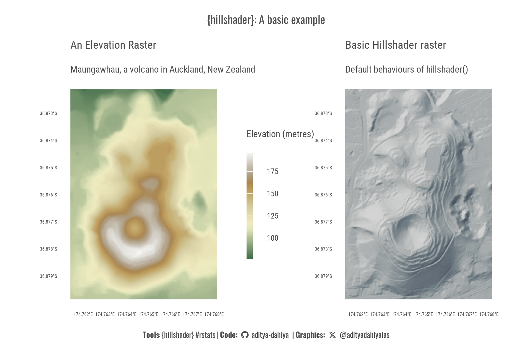
Exploring the {hillshader} package

The hillshader package (Roudier 2024) is an R tool designed to create shaded relief maps using ray-tracing techniques.t serves as a wrapper around the rayshader (Morgan-Wall 2024) and raster (Hijmans 2024) packages, facilitating the generation of hillshade relief maps and their export to spatial files.

The primary function, hillshader(), allows for the creation of hillshade maps as RasterLayer objects. Users can customize the shading process by specifying different shader functions, such as ray_shade and ambient_shade, and adjust parameters like sun angle and altitude to achieve desired visual effects. Additionally, the package offers functions like add_shadow_2d, matrix_to_raster, and write_raster to enhance integration with rayshader pipelines and GIS workflows.

# Data Import and Wrangling Tools
library(sf)                   # Handling simple features in R
library(terra)                # Handling rasters in R
library(tidyterra)            # Rasters with ggplot2
library(tidyverse)            # All things tidy

# Final plot tools
library(scales)               # Nice Scales for ggplot2
library(fontawesome)          # Icons display in ggplot2
library(ggtext)               # Markdown text in ggplot2
library(showtext)             # Display fonts in ggplot2
library(colorspace)           # Lighten and Darken colours
library(patchwork)            # Composing Plots

# Package to explore
library(rayshader)            # 2D / 3D map visualizations
library(raster)               # Handling rasters
library(hillshader)           # Shaded reliefs in R

# Making tables in R
library(gt)                   # Beautiful Tables

bts = 36 # Base Text Size
sysfonts::font_add_google("Roboto Condensed", "body_font")
sysfonts::font_add_google("Oswald", "title_font")
showtext::showtext_auto()
theme_set(
  theme_minimal(
    base_size = bts,
    base_family = "body_font"
  ) +
    theme(
      text = element_text(
        colour = "grey30",
        lineheight = 0.3,
        margin = margin(0,0,0,0, "pt")
      ),
      plot.title = element_text(
        hjust = 0.5
      ),
      plot.subtitle = element_text(
        hjust = 0.5
      )
    )
)

# Some basic caption stuff
# A base Colour
bg_col <- "white"
seecolor::print_color(bg_col)

# Colour for highlighted text
text_hil <- "grey30"
seecolor::print_color(text_hil)

# Colour for the text
text_col <- "grey20"
seecolor::print_color(text_col)


# Caption stuff for the plot
sysfonts::font_add(
  family = "Font Awesome 6 Brands",
  regular = here::here("docs", "Font Awesome 6 Brands-Regular-400.otf")
)
github <- "&#xf09b"
github_username <- "aditya-dahiya"
xtwitter <- "&#xe61b"
xtwitter_username <- "@adityadahiyaias"
social_caption_1 <- glue::glue("<span style='font-family:\"Font Awesome 6 Brands\";'>{github};</span> <span style='color: {text_hil}'>{github_username}  </span>")
social_caption_2 <- glue::glue("<span style='font-family:\"Font Awesome 6 Brands\";'>{xtwitter};</span> <span style='color: {text_hil}'>{xtwitter_username}</span>")
plot_caption <- paste0(
  "**Tools**: {hillshader} *#rstats* ",
  "  |  **Code:** ", 
  social_caption_1, 
  " |  **Graphics:** ", 
  social_caption_2
  )
rm(github, github_username, xtwitter, 
   xtwitter_username, social_caption_1, 
   social_caption_2)

Exploring the in-built data example

maungawhau_hr

hs <- hillshader(maungawhau_hr)

g1 <- ggplot() +
  geom_spatraster(data = rast(maungawhau_hr)) +
  scale_fill_wiki_c() +
  labs(
    title = "An Elevation Raster",
    subtitle = "Maungawhau, a volcano in Auckland, New Zealand",
    fill = "Elevation (metres)"
  ) +
  coord_sf(expand = F, clip = "off") +
  theme(
    panel.grid = element_blank(),
    legend.key.width = unit(5, "pt"),
    plot.margin = margin(0,0,0,5, "pt"),
    legend.margin = margin(0,0,0,0, "pt"),
    legend.box.margin = margin(0,0,0,0, "pt"),
    axis.text = element_text(size = bts/2)
  )

g2 <- ggplot() +
  geom_spatraster(data = rast(hs)) +
  paletteer::scale_fill_paletteer_c("ggthemes::Gray", -1) +
  labs(
    title = "Basic Hillshader raster",
    subtitle = "Default behaviours of hillshader()"
  ) +
  coord_sf(expand = F, clip = "off") +
  theme(
    legend.position = "none",
    panel.grid = element_blank(),
    plot.margin = margin(0,5,0,0, "pt"),
    axis.text = element_text(size = bts/2)
  )

g <- g1 + g2 +
  plot_annotation(
    title = "{hillshader}: A basic example",
    caption = plot_caption,
    theme = theme(
      plot.title = element_text(
        hjust = 0.5,
        family = "title_font"
      ),
      plot.caption = element_textbox(
        hjust = 0.5,
        family = "title_font"
      )
    )
  )

ggsave(
  plot = g,
  filename = here::here(
    "geocomputation", "images",
    "hillshader_package_1.png"
  ),
  height = 1200,
  width = 1800,
  units = "px",
  bg = "white"
)

Trying out an example: Himachal Pradesh with {elevatr} data

himachal_vec <- read_sf(
  here::here(
    "data", "india_map",
    "India_State_Boundary.shp"
  )
) |> 
  filter(State_Name == "Himachal Pradesh") |> 
  st_transform("EPSG:4326")

# ggplot(himachal_vec) +
#   geom_sf()
# 
# st_bbox(himachal_vec)

himachal_rast <- elevatr::get_elev_raster(
  locations = himachal_vec,
  z = 7
) |> 
  rast() |> 
  terra::crop(himachal_vec) |> 
  terra::mask(himachal_vec)

g1 <- ggplot() +
  geom_spatraster(data = himachal_rast) +
  geom_sf(data = himachal_vec, fill = NA) +
  scale_fill_wiki_c() +
  labs(
    title = "Himachal Pradesh (India)",
    fill = "Elevation (metres)"
  ) +
  theme(
    legend.position = "inside",
    legend.position.inside = c(0,0),
    legend.justification = c(0,0),
    legend.key.height = unit(10, "pt"),
    legend.title.position = "top",
    legend.direction = "horizontal",
    plot.title = element_text(
        size = bts * 2,
        margin = margin(15,0,2,0, "pt")
      ),
    panel.grid = element_line(
        linewidth = 0.2,
        linetype = 3
    )
  )

plot_himachal <- function(sunangle = 315, sunaltitude = 0){
  hs <- himachal_rast |> 
    raster() |> 
    hillshader(
      c("ray_shade", "ambient_shade"),
      sunangle = sunangle,
      sunaltitude = sunaltitude
    )

  ggplot() +
    geom_spatraster(data = rast(hs)) +
    geom_sf(data = himachal_vec, fill = NA) +
    paletteer::scale_fill_paletteer_c(
      "ggthemes::Classic Gray", 
      direction = 1,
      na.value = "transparent",
      trans = "log2"
    ) +
    labs(
      title = paste0("sunangle: ", sunangle, 
                     "  ; sunaltitude: ",
                     sunaltitude)
    ) +
    coord_sf(expand = F, clip = "off") +
    theme(
      legend.position = "none",
      panel.grid = element_line(
        linewidth = 0.2,
        linetype = 3
      ),
      plot.margin = margin(0,5,0,0, "pt"),
      axis.text = element_text(size = bts/2),
      plot.title = element_text(
        size = bts * 2,
        margin = margin(15,0,2,0, "pt")
      ),
      plot.subtitle = element_text(
        margin = margin(0,0,0,0, "pt")
      )
    )
}

g2 <- plot_himachal(sunangle = 315, sunaltitude = 0)

g3 <- plot_himachal(sunangle = 90, sunaltitude = 30)

g4 <- plot_himachal(sunangle = 315, sunaltitude = 30)

g5 <- plot_himachal(sunangle = 90, sunaltitude = 60)

g6 <- plot_himachal(sunangle = 315, sunaltitude = 60)

g <- wrap_plots(g1, g2, g3, g4, g5, g6) +
  plot_layout(
    ncol = 2,
    nrow = 3
  ) +
  plot_annotation(
    title = "Combinations of sun-angle & sun-altitude in {hillshader}",
    caption = plot_caption,
    theme = theme(
      plot.title = element_text(
        family = "title_font",
        size = bts * 3,
        hjust = 0.5,
        lineheight = 0.3,
        margin = margin(20,0,0,0, "pt")
      ),
      plot.caption = element_textbox(
        hjust = 0.5
      )
    )
  )

ggsave(
  plot = g,
  filename = here::here(
    "geocomputation", "images",
    "hillshader_package_2.png"
  ),
  height = 4800,
  width = 3600,
  units = "px",
  bg = "white"
)

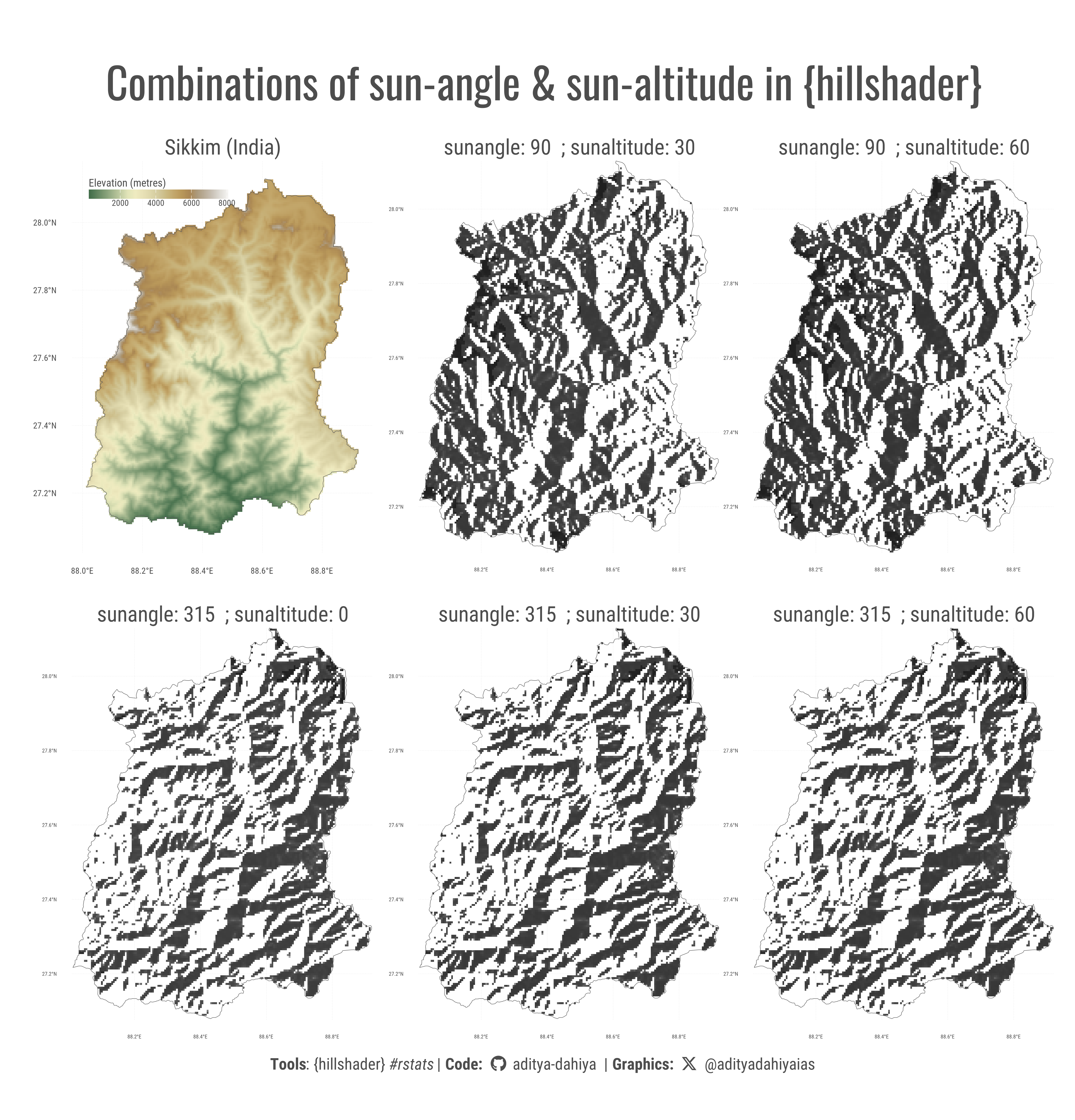
Another example for a smaller area - Sikkim (India)

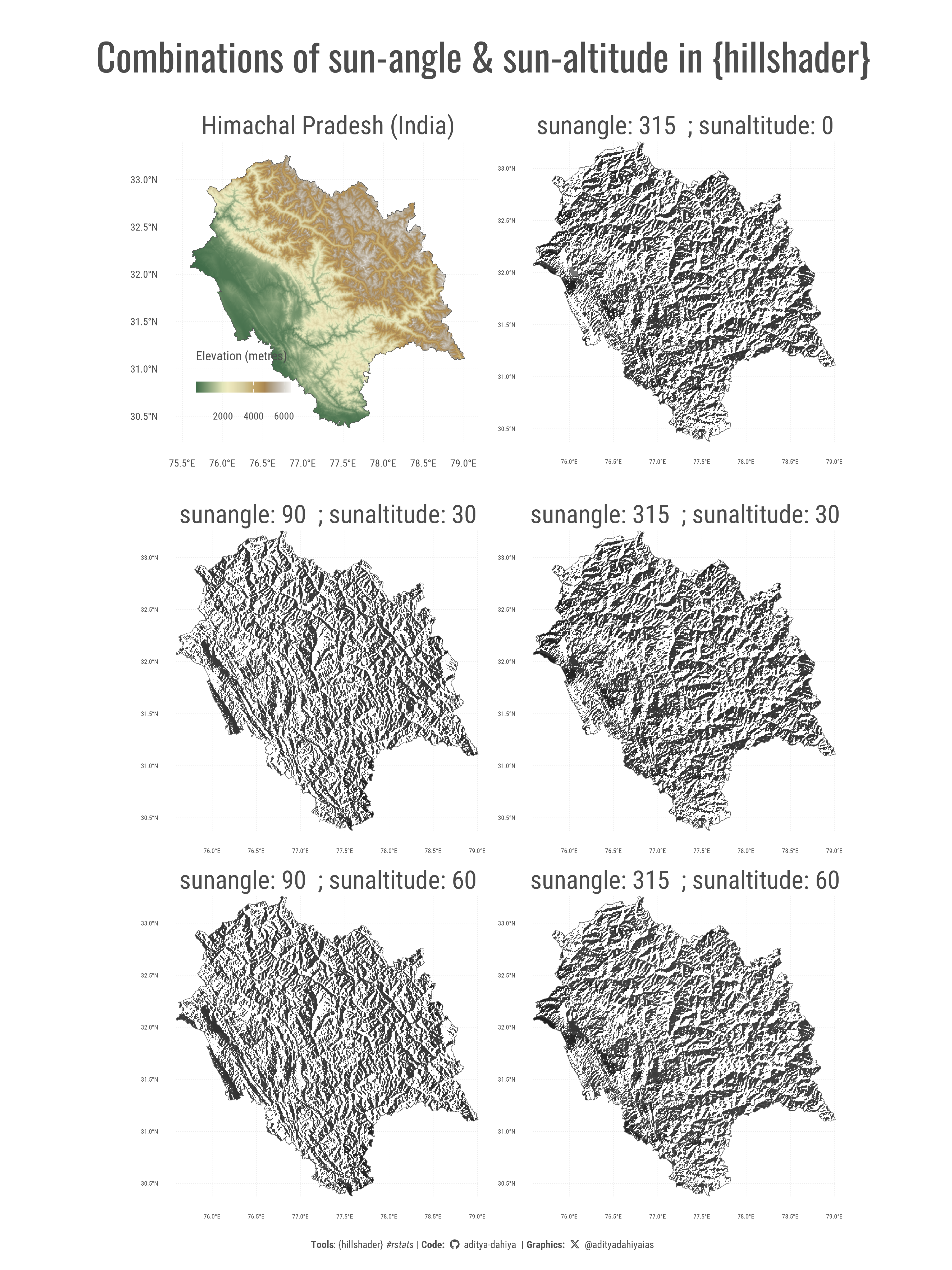
The analysis uses the hillshader package to generate five different hillshade maps of Sikkim, India, by varying the sunangle and sunaltitude parameters. The base map is created by extracting elevation data using elevatr::get_elev_raster() and masking it with the Sikkim state boundary from a shapefile loaded with sf::read_sf(). The function plot_sikkim() applies hillshader() with ray-traced shading techniques (ray_shade and ambient_shade) and visualizes the results using ggplot2::geom_spatraster() for a grayscale effect. Different combinations of sunlight direction (sunangle) and height (sunaltitude) alter the relief perception. The six maps, including an elevation reference, are arranged with patchwork::wrap_plots(), demonstrating how terrain visualization changes under varying lighting conditions.

sikkim_vec <- read_sf(
  here::here(
    "data", "india_map",
    "India_State_Boundary.shp"
  )
) |> 
  filter(State_Name == "Sikkim") |> 
  st_transform("EPSG:4326")

ggplot(sikkim_vec) +
  geom_sf()

st_bbox(sikkim_vec)

sikkim_rast <- elevatr::get_elev_raster(
  locations = sikkim_vec,
  z = 7
) |> 
  rast() |> 
  terra::crop(sikkim_vec) |> 
  terra::mask(sikkim_vec)

g1 <- ggplot() +
  geom_spatraster(data = sikkim_rast) +
  geom_sf(data = sikkim_vec, fill = NA) +
  scale_fill_wiki_c() +
  labs(
    title = "Sikkim (India)",
    fill = "Elevation (metres)"
  ) +
  theme(
    legend.position = "inside",
    legend.position.inside = c(0,1),
    legend.justification = c(0,1),
    legend.key.height = unit(10, "pt"),
    legend.key.width = unit(30, "pt"),
    legend.title.position = "top",
    legend.direction = "horizontal",
    plot.title = element_text(
        size = bts * 2,
        margin = margin(15,0,2,0, "pt")
      ),
    panel.grid = element_line(
        linewidth = 0.2,
        linetype = 3
    ),
    legend.title = element_text(
      margin = margin(0,0,2,0, "pt")
    ),
    legend.text = element_text(
      margin = margin(1,0,0,0, "pt")
    )
  )

plot_sikkim <- function(sunangle = 315, sunaltitude = 0){
  hs <- sikkim_rast |> 
    raster() |> 
    hillshader(
      c("ray_shade", "ambient_shade"),
      sunangle = sunangle,
      sunaltitude = sunaltitude
    )

  ggplot() +
    geom_spatraster(data = rast(hs)) +
    geom_sf(data = sikkim_vec, fill = NA) +
    paletteer::scale_fill_paletteer_c(
      "ggthemes::Classic Gray", 
      direction = 1,
      na.value = "transparent",
      trans = "log2"
    ) +
    labs(
      title = paste0("sunangle: ", sunangle, 
                     "  ; sunaltitude: ",
                     sunaltitude)
    ) +
    coord_sf(expand = F, clip = "off") +
    theme(
      legend.position = "none",
      panel.grid = element_line(
        linewidth = 0.2,
        linetype = 3
      ),
      plot.margin = margin(0,5,0,0, "pt"),
      axis.text = element_text(size = bts/2),
      plot.title = element_text(
        size = bts * 2,
        margin = margin(15,0,2,0, "pt")
      ),
      plot.subtitle = element_text(
        margin = margin(0,0,0,0, "pt")
      )
    )
}

g2 <- plot_sikkim(sunangle = 315, sunaltitude = 0)

g3 <- plot_sikkim(sunangle = 90, sunaltitude = 30)

g4 <- plot_sikkim(sunangle = 315, sunaltitude = 30)

g5 <- plot_sikkim(sunangle = 90, sunaltitude = 60)

g6 <- plot_sikkim(sunangle = 315, sunaltitude = 60)

g <- wrap_plots(g1, g3, g5, g2, g4, g6) +
  plot_layout(
    ncol = 3,
    nrow = 2
  ) +
  plot_annotation(
    title = "Combinations of sun-angle & sun-altitude in {hillshader}",
    caption = plot_caption,
    theme = theme(
      plot.title = element_text(
        family = "title_font",
        size = bts * 4,
        hjust = 0.5,
        lineheight = 0.3,
        margin = margin(20,0,0,0, "pt")
      ),
      plot.caption = element_textbox(
        hjust = 0.5,
        size = bts * 1.5
      )
    )
  )

ggsave(
  plot = g,
  filename = here::here(
    "geocomputation", "images",
    "hillshader_package_3.png"
  ),
  height = 5000,
  width = 4800,
  units = "px",
  bg = "white"
)

This visualization showcases the impact of varying sun angles and altitudes on hillshade maps of Sikkim, India, using the {hillshader} package. The top-left map represents the original elevation data, while the remaining five maps illustrate different shading effects based on changes in sunangle (direction of sunlight) and sunaltitude (height of the sun above the horizon). By adjusting these parameters, the perception of terrain depth and structure changes, highlighting how light sources influence the visualization of topography.

References

Hijmans, Robert J. 2024. “Raster: Geographic Data Analysis and Modeling.” https://CRAN.R-project.org/package=raster.

Morgan-Wall, Tyler. 2024. “Rayshader: Create Maps and Visualize Data in 2D and 3D.” https://CRAN.R-project.org/package=rayshader.

Roudier, Pierre. 2024. “Hillshader: Create Hillshade Relief Maps Using Ray-Tracing.” https://CRAN.R-project.org/package=hillshader.