Code
pacman::p_load(
  sf,
  terra,
  tidyterra,

  tidyverse,

  ggplot2,
  showtext,
  scales,
  ggtext,
  fontawesome,

  geodata,
  ggmap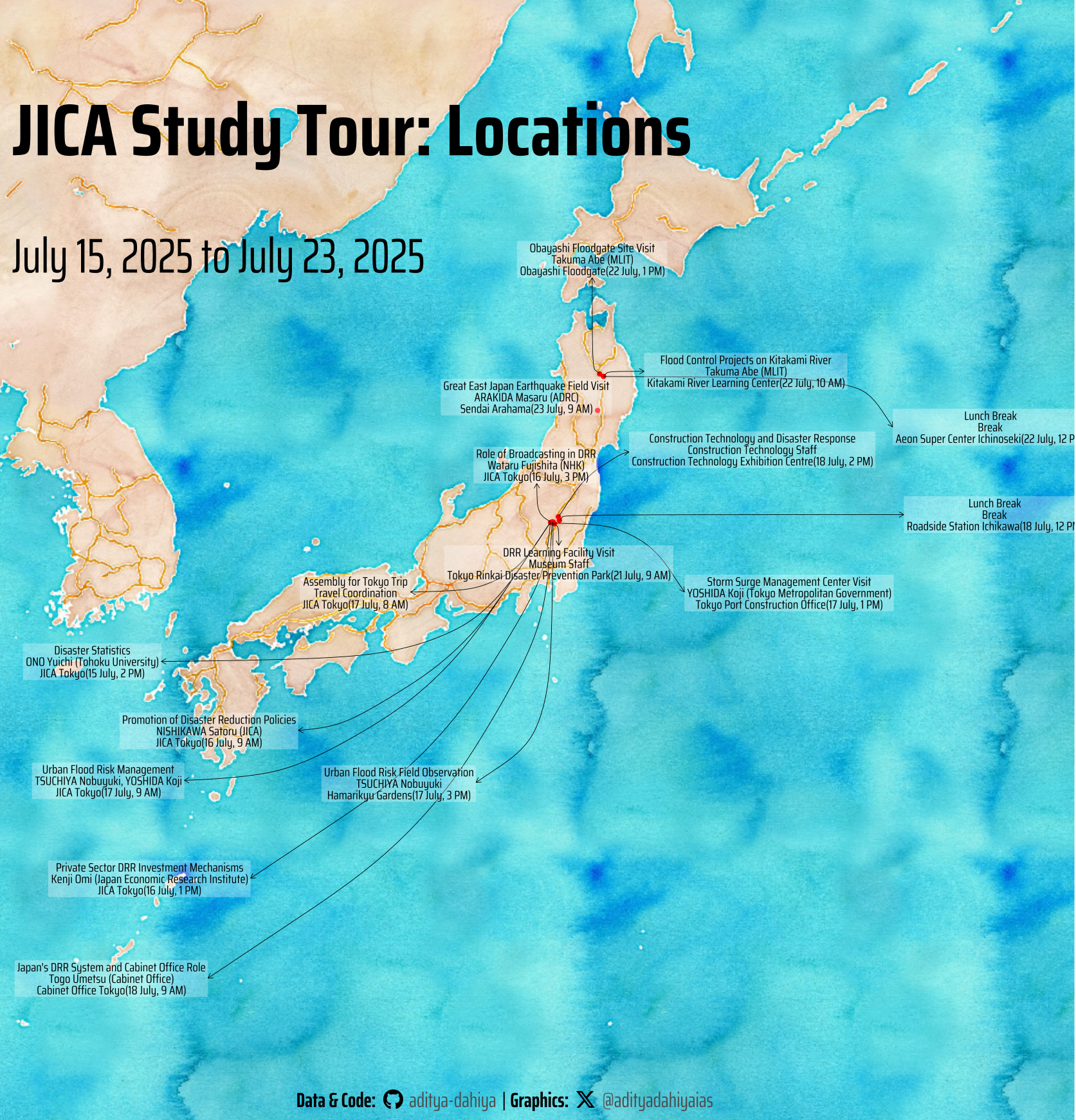
)A spatiotemporal visualization of key locations and sessions from the July 2025 JICA Disaster Risk Reduction training program across Japan
This map was created in R using the {ggplot2} framework, enhanced by a suite of geospatial and visualization packages. I began by parsing the JICA training calendar in .ics format using {ical} and transformed the schedule into a tidy table using {lubridate} and {tidyverse}. Location names were geocoded via the OpenStreetMap Nominatim API using {tidygeocoder} and converted to spatial features with {sf}. To provide geographic context, I used {rnaturalearth} for Japan’s administrative boundaries and overlaid watercolor tiles from {ggmap} via {terra} and {tidyterra} for raster integration. Labels were dynamically placed with {ggrepel}, and visual styling was refined using {ggtext}, {showtext}, and Google Fonts. The final composition brings together aesthetics and information design to trace the journey from Tokyo to Sendai, offering a visual record of the immersive disaster risk reduction sessions undertaken during the program.
pacman::p_load(
sf,
terra,
tidyterra,
tidyverse,
ggplot2,
showtext,
scales,
ggtext,
fontawesome,
geodata,
ggmap
)# Visualization Parameters
bts = 12 # Base Text Size
sysfonts::font_add_google("Saira Condensed", "body_font")
sysfonts::font_add_google("Saira", "title_font")
sysfonts::font_add_google("Saira Extra Condensed", "caption_font")
showtext::showtext_auto()
# A base Colour
bg_col <- "white"
seecolor::print_color(bg_col)
# Colour for highlighted text
text_hil <- "grey30"
seecolor::print_color(text_hil)
# Colour for the text
text_col <- "grey20"
seecolor::print_color(text_col)
theme_set(
theme_minimal(
base_size = bts,
base_family = "body_font"
) +
theme(
text = element_text(
colour = "grey30",
lineheight = 0.3,
margin = margin(0,0,0,0, "pt")
),
plot.title = element_text(
hjust = 0.5
),
plot.subtitle = element_text(
hjust = 0.5
)
)
)
# Caption stuff for the plot
sysfonts::font_add(
family = "Font Awesome 6 Brands",
regular = here::here("docs", "Font Awesome 6 Brands-Regular-400.otf")
)
github <- ""
github_username <- "aditya-dahiya"
xtwitter <- ""
xtwitter_username <- "@adityadahiyaias"
social_caption_1 <- glue::glue("<span style='font-family:\"Font Awesome 6 Brands\";'>{github};</span> <span style='color: {text_hil}'>{github_username} </span>")
social_caption_2 <- glue::glue("<span style='font-family:\"Font Awesome 6 Brands\";'>{xtwitter};</span> <span style='color: {text_hil}'>{xtwitter_username}</span>")
plot_caption <- paste0(
"**Data & Code:** ",
social_caption_1,
" | **Graphics:** ",
social_caption_2
)
rm(github, github_username, xtwitter,
xtwitter_username, social_caption_1,
social_caption_2)
size_var <- 9000
bts = 150Get JICA Data (ChatGPT) attempt
# Load necessary libraries
library(tidyverse)
library(ical)
library(lubridate)
library(tidygeocoder)
library(sf)

# Step 1: Read the .ics file
ics_data <- ical_parse_df(
  "C:/Users/dradi/Downloads/JICA Official Schedule_4684d7f0594c3cb3308127b6d5cf7f6990db74baed3882549c5c535e64084868@group.calendar.google.com.ics"
) |>
  as_tibble()

# Step 2: Filter only VEVENT types
# events <- ics_data %>%
#   filter(component == "VEVENT")

# Create initial tibble with parsed columns
calendar_tbl <- ics_data |>
  transmute(
    date_time = as_datetime(start),
    date = as_date(start),
    time = format(as_datetime(start), "%H:%M"),
    topic_of_meeting = summary,
    # location = str_remove(location, ",.*"),  # Keep only place name
    lecturer = str_extract(description, "(?<=Lecturer\\(s\\): ).*"),
    description = description
  )

# Step 4: Geocode location (Place Name Only)
calendar_tbl <- calendar_tbl %>%
  mutate(location_clean = if_else(is.na(location), NA_character_, location)) %>%
  geocode(location_clean, method = "osm", lat = latitude, long = longitude)

# Step 5: Convert to sf POINT object
calendar_sf <- calendar_tbl %>%
  filter(!is.na(latitude) & !is.na(longitude)) %>%
  st_as_sf(coords = c("longitude", "latitude"), crs = 4326)

# Step 6: Add geometry column and display tibble
calendar_sf <- calendar_sf %>%
  select(date, time, date_time, location, geometry, topic_of_meeting, lecturer, description)

# View the tibble
print(calendar_sf)
Getting JICA Study Tour Data (Claude AI attempt)
library(tidyverse)
library(sf)
library(lubridate)

# Create tibble with JICA events from July 15-23, 2025
jica_events <- tibble(
  date = as.Date(c(
    "2025-07-15", "2025-07-16", "2025-07-16", "2025-07-16", "2025-07-16",
    "2025-07-17", "2025-07-17", "2025-07-17", "2025-07-18", "2025-07-18",
    "2025-07-18", "2025-07-21", "2025-07-22", "2025-07-22", "2025-07-22", "2025-07-23"
  )),

  time = c(
    "14:00-17:00", "09:00-12:00", "13:30-14:30", "15:00-16:45", "08:30-09:30",
    "09:30-11:30", "13:30-14:45", "15:15-17:30", "09:30-11:30", "12:00-13:00",
    "14:00-15:30", "09:30-11:00", "10:00-12:00", "12:30-13:00", "13:00-15:00", "09:30-14:20"
  ),

  date_time = as.POSIXct(c(
    "2025-07-15 14:00:00", "2025-07-16 09:00:00", "2025-07-16 13:30:00",
    "2025-07-16 15:00:00", "2025-07-17 08:30:00", "2025-07-17 09:30:00",
    "2025-07-17 13:30:00", "2025-07-17 15:15:00", "2025-07-18 09:30:00",
    "2025-07-18 12:00:00", "2025-07-18 14:00:00", "2025-07-21 09:30:00",
    "2025-07-22 10:00:00", "2025-07-22 12:30:00", "2025-07-22 13:00:00", "2025-07-23 09:30:00"
  ), tz = "Asia/Tokyo"),

  location = c(
    "JICA Tokyo", "JICA Tokyo", "JICA Tokyo", "JICA Tokyo", "JICA Tokyo",
    "JICA Tokyo", "Tokyo Port Construction Office", "Hamarikyu Gardens",
    "Cabinet Office Tokyo", "Roadside Station Ichikawa", "Construction Technology Exhibition Centre",
    "Tokyo Rinkai Disaster Prevention Park", "Kitakami River Learning Center",
    "Aeon Super Center Ichinoseki", "Obayashi Floodgate", "Sendai Arahama"
  ),

  topic_of_meeting = c(
    "Disaster Statistics", "Promotion of Disaster Reduction Policies",
    "Private Sector DRR Investment Mechanisms", "Role of Broadcasting in DRR",
    "Assembly for Tokyo Trip", "Urban Flood Risk Management",
    "Storm Surge Management Center Visit", "Urban Flood Risk Field Observation",
    "Japan's DRR System and Cabinet Office Role", "Lunch Break",
    "Construction Technology and Disaster Response", "DRR Learning Facility Visit",
    "Flood Control Projects on Kitakami River", "Lunch Break",
    "Obayashi Floodgate Site Visit", "Great East Japan Earthquake Field Visit"
  ),

  lecturer = c(
    "ONO Yuichi (Tohoku University)", "NISHIKAWA Satoru (JICA)",
    "Kenji Omi (Japan Economic Research Institute)", "Wataru Fujishita (NHK)",
    "Travel Coordination", "TSUCHIYA Nobuyuki, YOSHIDA Koji",
    "YOSHIDA Koji (Tokyo Metropolitan Government)", "TSUCHIYA Nobuyuki",
    "Togo Umetsu (Cabinet Office)", "Break",
    "Construction Technology Staff", "Museum Staff",
    "Takuma Abe (MLIT)", "Break",
    "Takuma Abe (MLIT)", "ARAKIDA Masaru (ADRC)"
  ),

  event_type = c(
    "Lecture", "Lecture", "Lecture", "Lecture", "Travel",
    "Lecture", "Observation", "Observation", "Lecture", "Break",
    "Observation", "Observation", "Lecture", "Break", "Observation", "Observation"
  ),

  venue_detail = c(
    "SR 402 Main Building", "SR 402 Main Building", "SR 402 Main Building",
    "SR 402 Main Building", "JICA Tokyo", "JICA Tokyo",
    "Storm Surge Management Center", "Hamarikyu Imperial Garden",
    "Government Office Complex No. 8", "Ichikawa", "Matsudo Chiba",
    "Ariake Tokyo", "Ichinoseki Iwate", "Ichinoseki Iwate",
    "Kitakami River", "Arahama Elementary School"
  )
)

# Create geometry column with sf POINT objects
# Coordinates are approximate based on location names
coords <- tibble(
  location = c(
    "JICA Tokyo", "JICA Tokyo", "JICA Tokyo", "JICA Tokyo", "JICA Tokyo",
    "JICA Tokyo", "Tokyo Port Construction Office", "Hamarikyu Gardens",
    "Cabinet Office Tokyo", "Roadside Station Ichikawa", "Construction Technology Exhibition Centre",
    "Tokyo Rinkai Disaster Prevention Park", "Kitakami River Learning Center",
    "Aeon Super Center Ichinoseki", "Obayashi Floodgate", "Sendai Arahama"
  ),
  lon = c(
    139.6917, 139.6917, 139.6917, 139.6917, 139.6917,
    139.6917, 139.7514, 139.7638, 139.7414, 139.9308, 139.9023,
    139.7967, 141.1347, 141.1347, 141.0283, 140.9736
  ),
  lat = c(
    35.6612, 35.6612, 35.6612, 35.6612, 35.6612,
    35.6612, 35.6508, 35.6692, 35.6751, 35.7089, 35.7878,
    35.6331, 38.9275, 38.9275, 38.9833, 38.1661
  )
)

# Add geometry column as sf points
jica_events <- jica_events |>
  left_join(coords, by = "location", relationship = "many-to-many")  |>
  st_as_sf(coords = c("lon", "lat"), crs = 4326) |>
  distinct() |>
  mutate(
    formatted_datetime_alt = format(date_time, "%d %B, %I %p") |>
      str_replace("^0", "") |>   # Remove leading zero from day
      # str_to_lower() |>          # Convert AM/PM to lowercase
      str_replace(" 0", " ")     # Remove leading zero from hour if present
  ) |>
  mutate(
    nudge_x_var = if_else(
      date >= as_date("2025-07-21"),
      -2,
      2
    )
  )

# Test Check
ggplot(jica_events) +
  geom_sf()
Get Japan Base Map
base_map_1 <- rnaturalearth::ne_countries(
  country = "Japan",
  scale = "large"
) |>
  select(geometry)


library(sf)

# Extract bounding box from your sf object
japan_bbox <- st_bbox(base_map_1)

# Convert to named vector in the format you requested
japan_bbox <- c(
  left = japan_bbox[["xmin"]],
  bottom = japan_bbox[["ymin"]] - 2,
  right = japan_bbox[["xmax"]],
  top = japan_bbox[["ymax"]] + 2
)

base_map_2 <- get_stadiamap(
  bbox = japan_bbox,
  zoom = 7,
  maptype = "stamen_watercolor"
)

base_map_rast <- base_map_2 |>
  rast()

# ggplot() +
#   geom_spatraster_rgb(
#     data = base_map_rast
#   )
Plot the Map
base_map_1 |>
  ggplot() +
geom_sf(data = base_map_1) +
  geom_sf(
    data = jica_events,
    size = 4,
    alpha = 3,
    colour = "red"
  )

g <- base_map_1 |>
  ggplot() +
  geom_sf(data = base_map_1) +
  geom_spatraster_rgb(
    data = base_map_rast,
    maxcell = 1e6
  ) +
  geom_sf(
    data = jica_events,
    size = 4,
    alpha = 3,
    colour = "red"
  ) +
  ggrepel::geom_label_repel(
    data = jica_events,
    mapping = aes(
      label = paste0(
        topic_of_meeting,
        "\n",
        lecturer,
        "\n",
        location, "(",
        formatted_datetime_alt,
        ")"
      ),
      geometry = geometry
    ),
    stat = "sf_coordinates",
    force = 100,
    force_pull = 0.01,
    max.overlaps = 100,
    lineheight = 0.25,
    size = 25,
    family = "body_font",
    arrow = arrow(
      length = unit(10, "pt"),
      ends = "first"
    ),
    fill = alpha("white", 0.3),
    label.padding = unit(5, "pt"),
    max.iter = 10,
    label.size = NA,
    segment.curvature = 0.2,
    segment.size = 0.5,
    xlim = c(125, 155),
    ylim = c(25, 42),
    seed = 42
  ) +
  coord_sf(
    expand = FALSE
  ) +
  annotate(
    geom = "text",
    label = "JICA Study Tour: Locations",
    x = 125, y = 45,
    hjust = 0,
    vjust = 1,
    size = bts,
    family = "body_font",
    fontface = "bold"
    # fill = alpha("white", 0.4),
    # label.r = unit(10, "pt"),
    # label.size = NA
  ) +
  annotate(
    geom = "text",
    label = "July 15, 2025 to July 23, 2025",
    x = 125, y = 42,
    hjust = 0,
    vjust = 1,
    size = bts / 1.5,
    family = "caption_font",
    # fill = alpha("white", 0.4),
    fontface = "italic"
    # label.r = unit(10, "pt"),
    # lineheight = 0.3,
    # label.size = NA
  ) +
  labs(
    caption = plot_caption
  ) +
  ggthemes::theme_map(
    base_size = bts,
    base_family = "body_font"
  ) +
  theme(
    plot.caption = element_textbox(
      halign = 0.5,
      hjust = 0.5,
      family = "caption_font",
      margin = margin(-100,0,0,0, "pt")
    ),
    plot.title = element_text(
      margin = margin(10,0,10,0, "pt"),
      hjust = 0.5
    ),
    plot.subtitle = element_text(
      margin = margin(0,0,0,0, "pt"),
      hjust = 0.5
    ),
    plot.margin = margin(0,0,0,0, "pt")
  )


ggsave(
  plot = g,
  filename = here::here("geocomputation",
                        "images",
                        "jica_study_tour_1.png"),
  width = size_var,
  height = size_var,
  units = "px",
  bg = bg_col
)