Different Packages to access Open Street Maps in R

Exploring {osmdata}, {osmextract}, {osmapiR}

Introduction

# Data wrangling & visualization
library(tidyverse)  # Data manipulation & visualization

# Spatial data handling
library(sf)         # Import, export, and manipulate vector data
library(terra)      # Import, export, and manipulate raster data

# ggplot2 extensions
library(tidyterra)  # Helper functions for using terra with ggplot2

# Final plot tools
library(scales)               # Nice Scales for ggplot2
library(fontawesome)          # Icons display in ggplot2
library(ggtext)               # Markdown text in ggplot2
library(showtext)             # Display fonts in ggplot2
library(patchwork)            # Composing Plots

bts = 42 # Base Text Size
sysfonts::font_add_google("Roboto Condensed", "body_font")
sysfonts::font_add_google("Oswald", "title_font")
sysfonts::font_add_google("Saira Extra Condensed", "caption_font")
showtext::showtext_auto()
# A base Colour
bg_col <- "white"
seecolor::print_color(bg_col)

# Colour for highlighted text
text_hil <- "grey30"
seecolor::print_color(text_hil)

# Colour for the text
text_col <- "grey20"
seecolor::print_color(text_col)

theme_set(
  theme_minimal(
    base_size = bts,
    base_family = "body_font"
  ) +
    theme(
      text = element_text(
        colour = "grey30",
        lineheight = 0.3,
        margin = margin(0,0,0,0, "pt")
      ),
      plot.title = element_text(
        hjust = 0.5
      ),
      plot.subtitle = element_text(
        hjust = 0.5
      )
    )
)

# Caption stuff for the plot
sysfonts::font_add(
  family = "Font Awesome 6 Brands",
  regular = here::here("docs", "Font Awesome 6 Brands-Regular-400.otf")
)
github <- "&#xf09b"
github_username <- "aditya-dahiya"
xtwitter <- "&#xe61b"
xtwitter_username <- "@adityadahiyaias"
social_caption_1 <- glue::glue("<span style='font-family:\"Font Awesome 6 Brands\";'>{github};</span> <span style='color: {text_hil}'>{github_username}  </span>")
social_caption_2 <- glue::glue("<span style='font-family:\"Font Awesome 6 Brands\";'>{xtwitter};</span> <span style='color: {text_hil}'>{xtwitter_username}</span>")
plot_caption <- paste0(
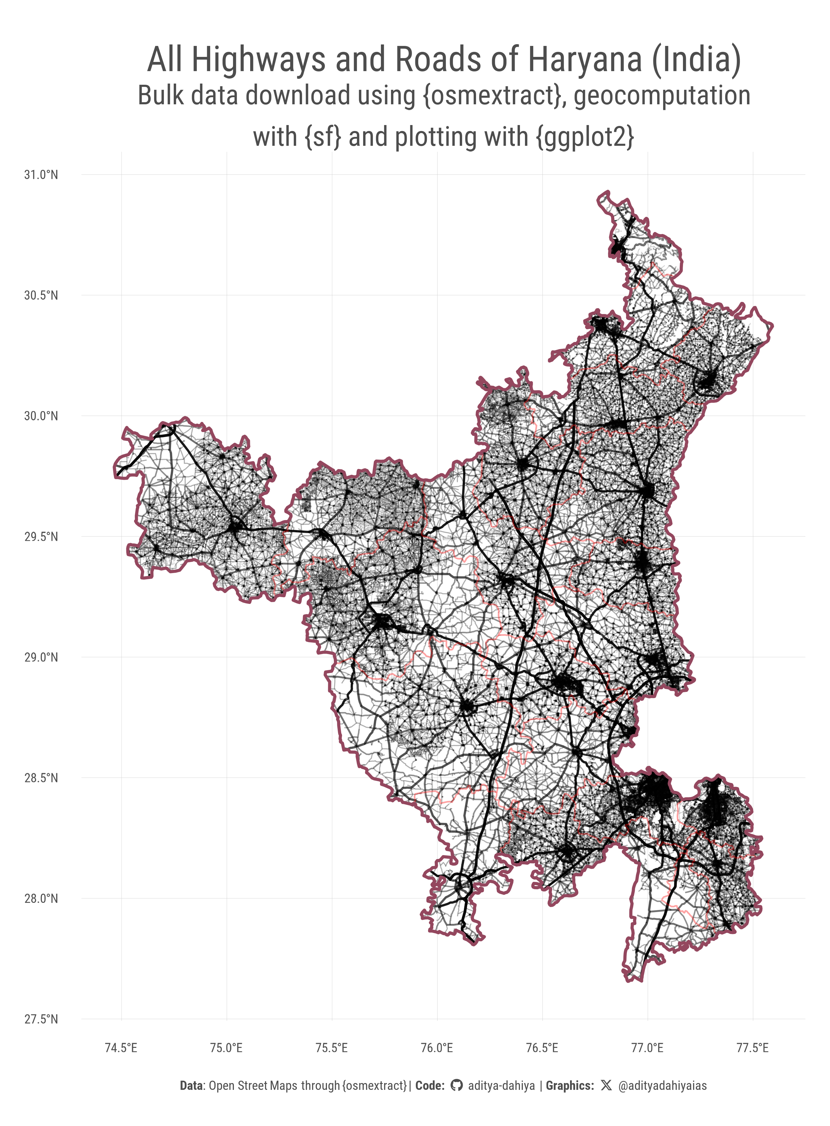
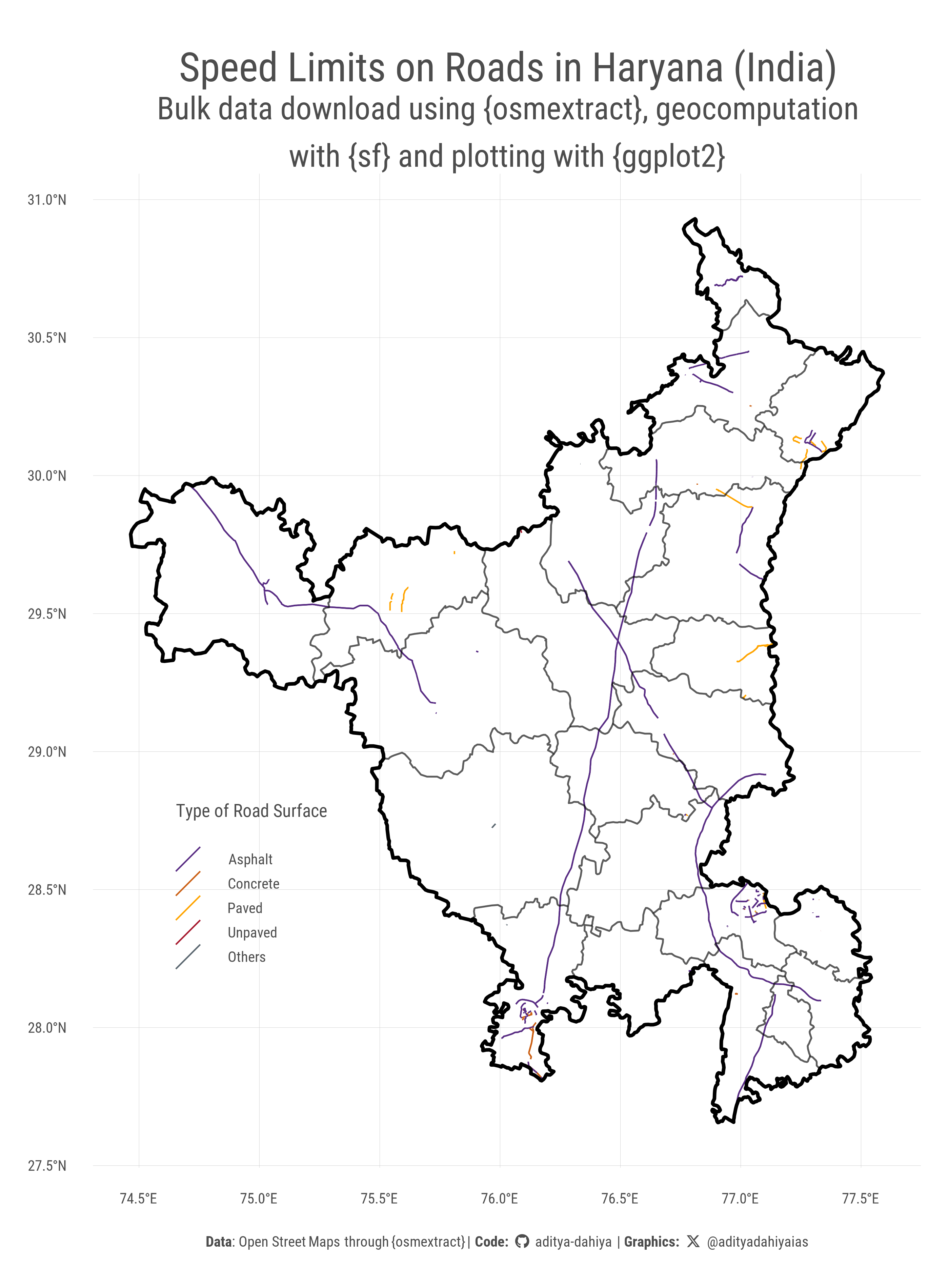
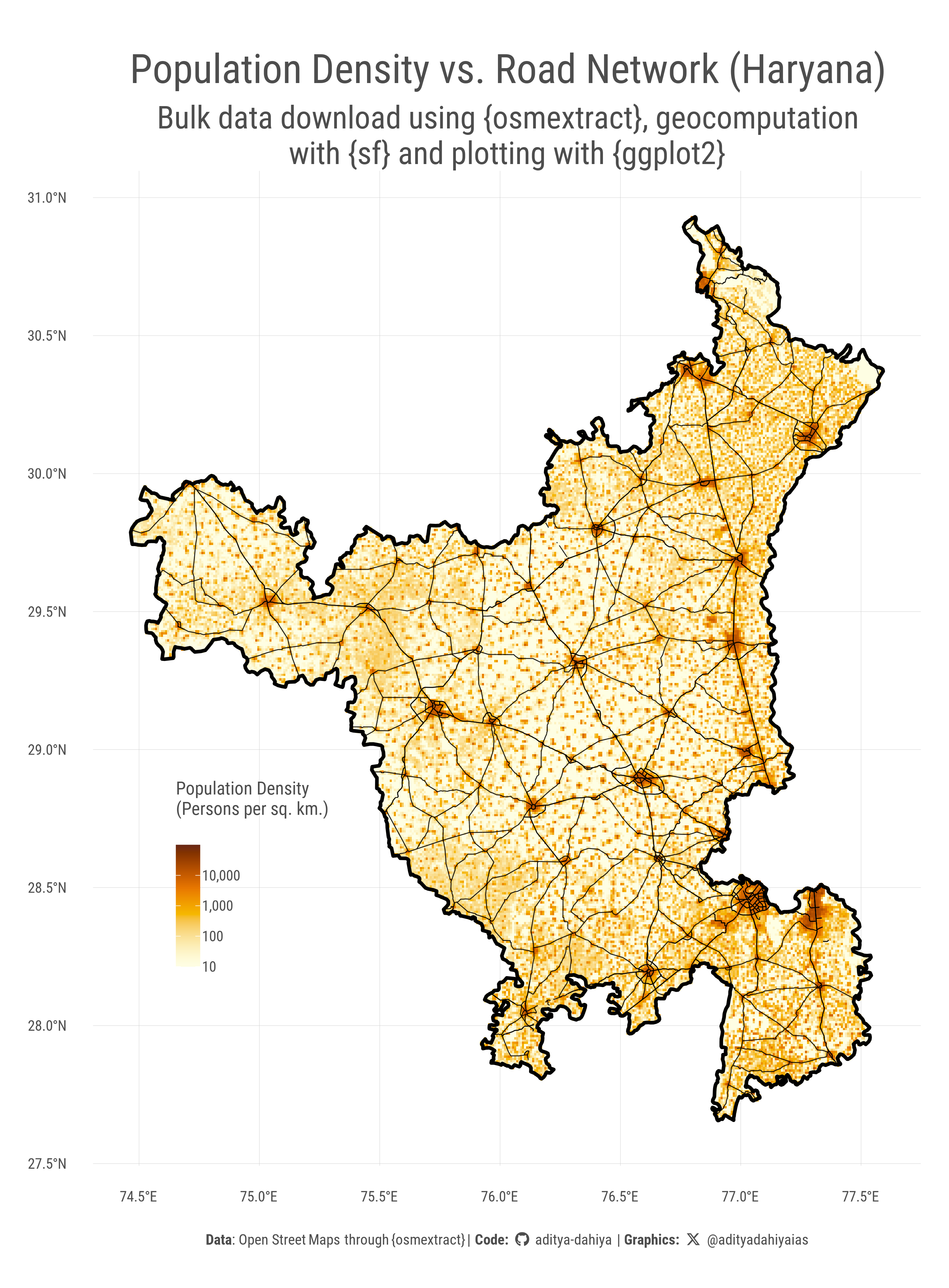
  "**Data**:  Open Street Maps through {osmextract}",
  "  |  **Code:** ", 
  social_caption_1, 
  " |  **Graphics:** ", 
  social_caption_2
  )
rm(github, github_username, xtwitter, 
   xtwitter_username, social_caption_1, 
   social_caption_2)

library(gt)

osm_packages <- tibble::tibble(
  `Package Name` = c(
    "[osmdata](https://github.com/ropensci/osmdata)",
    "[osmapiR](https://github.com/ropensci/osmapiR)",
    "[osmextract](https://github.com/ropensci/osmextract)",
    "[geofabrik](https://cran.r-project.org/package=geofabrik)"
  ),
  `Description` = c(
    "Provides an R interface to the Overpass API for querying OSM data.",
    "R interface to the OpenStreetMap API v0.6 for fetching and saving raw geodata.",
    "Downloads, converts, and imports bulk OSM data (.pbf files).",
    "Downloads OSM data from Geofabrik’s regional extracts."
  ),
  `Advantages` = c(
    "Ideal for extracting specific features; flexible Overpass API queries.",
    "Allows fetching, editing, and saving OSM data, including metadata and GPS traces.",
    "Efficiently handles large-scale OSM extracts; supports bulk processing.",
    "Easy access to pre-processed regional OSM extracts; simplifies data handling."
  ),
  `Disadvantages` = c(
    "Rate-limited API; not suited for large datasets.",
    "Not designed for bulk OSM data retrieval; more useful for metadata analysis.",
    "Requires handling large .pbf files; needs external dependencies for conversion.",
    "Limited to available regional extracts; lacks fine-grained filtering."
  )
)

osm_packages |> 
  gt() |> 
  gtExtras::gt_theme_nytimes() |> 
  fmt_markdown(columns = `Package Name`) |> 
  tab_header(
    title = "Comparison of R Packages for Accessing OpenStreetMap Data"
  ) |> 
  tab_footnote(
    footnote = md("**Data sources:** OpenStreetMap, Overpass API, Geofabrik, and various R package repositories.")
  ) |> 
  tab_style(
    style = cell_text(font = "monospace", weight = "bold"),
    locations = cells_body(
      columns = `Package Name`
    )
  )

Table 1: Comparison of various R packages that facilitate access to OpenStreetMap (OSM) data. Each package serves different purposes, ranging from querying small datasets via the Overpass API to downloading large-scale extracts for bulk processing.

Comparison of R Packages for Accessing OpenStreetMap Data
Package Name	Description	Advantages	Disadvantages
osmdata	Provides an R interface to the Overpass API for querying OSM data.	Ideal for extracting specific features; flexible Overpass API queries.	Rate-limited API; not suited for large datasets.
osmapiR	R interface to the OpenStreetMap API v0.6 for fetching and saving raw geodata.	Allows fetching, editing, and saving OSM data, including metadata and GPS traces.	Not designed for bulk OSM data retrieval; more useful for metadata analysis.
osmextract	Downloads, converts, and imports bulk OSM data (.pbf files).	Efficiently handles large-scale OSM extracts; supports bulk processing.	Requires handling large .pbf files; needs external dependencies for conversion.
geofabrik	Downloads OSM data from Geofabrik’s regional extracts.	Easy access to pre-processed regional OSM extracts; simplifies data handling.	Limited to available regional extracts; lacks fine-grained filtering.
Data sources: OpenStreetMap, Overpass API, Geofabrik, and various R package repositories.

osmextract

The {osmextract} package in R provides an efficient way to download and extract OpenStreetMap (OSM) data in a structured format. It allows users to retrieve spatial data such as points, lines, and polygons for specific geographic regions, making it useful for mapping, geospatial analysis, and urban studies. The package integrates well with {sf} to handle spatial objects and supports various file formats for seamless data extraction.

In the code provided, {osmextract} is used to fetch OSM data for Haryana in three layers: points, lines, and polygons. The {sf} package is used to manage and manipulate spatial vector data, converting extracted data into simple features. {geodata} helps in retrieving administrative boundaries from the GADM database.

# Load necessary libraries
library(osmextract)
library(sf)

# Download and extract the data
# Points
points_haryana <- oe_get(
  place = "Haryana",
  layer = "points",
  download_directory = "C:/Users/dradi/Desktop" 
)
object.size(points_haryana) |> print(units = "Mb")

# Lines
lines_haryana <- oe_get(
  place = "Haryana",
  layer = "lines",
  download_directory = "C:/Users/dradi/Desktop"
)
object.size(lines_haryana) |> print(units = "Mb")
# Polygons
polygons_haryana <- oe_get(
  place = "Haryana",
  layer = "multipolygons",
  download_directory = "C:/Users/dradi/Desktop"
)
object.size(polygons_haryana) |> print(units = "Mb")

# Get Haryana Map from GADM / {geodata} with geodata::gadm()
# District Wise Map
haryana_map <- geodata::gadm(
  country = "India",
  level = 2,
  path = tempdir()
) |> 
  st_as_sf() |> 
  janitor::clean_names() |> 
  filter(name_1 == "Haryana") |> 
  rename(district = name_2) |> 
  select(district, geometry)

# Overall Boundary Map
haryana_boundary <- geodata::gadm(
  country = "India",
  level = 1,
  path = tempdir()
) |> 
  st_as_sf() |> 
  janitor::clean_names() |> 
  filter(name_1 == "Haryana") |> 
  select(geometry)

Canals of Haryana

In this analysis, additional packages are used to enhance data extraction, processing, and visualization. The {elevatr} package is utilized to retrieve elevation raster data for Haryana. The {stringr} package is employed to extract numeric values from text-based attributes, such as canal width from OSM tags. The {tidyterra} package is indirectly referenced through geom_spatraster(), facilitating the inclusion of raster elevation data. Additionally, {sf} remains central for spatial vector data processing, and {geodata} continues to provide administrative boundaries from the GADM database. The final map effectively presents Haryana’s irrigation canal network overlaid on an elevation raster with clear administrative boundaries.

st_crs(points_haryana)

# Background raster for Haryana
# world_cbhsr_rast <- rnaturalearth::ne_download(
#   scale = 50,
#   type = "HYP_50M_SR",
#   category = "raster"
# )

raster_haryana <- elevatr::get_elev_raster(
  locations = haryana_boundary,
  z = 9
) |> 
  terra::rast() |> 
  terra::crop(haryana_boundary) |> 
  terra::mask(haryana_boundary)

canals_haryana <- lines_haryana |> 
  filter(waterway == "canal") |> 
  select(osm_id, name, other_tags, geometry) |> 
  mutate(width = str_extract(
    other_tags, '(?<=\\"width\\"=>\\")\\d+(?=\\")'),
    width = parse_number(width)
  ) |> 
  st_intersection(haryana_boundary)

g <- ggplot() +
  geom_spatraster(
    data = raster_haryana
  ) +
  scale_fill_gradient(
    high = "grey0", 
    low = "grey90",
    na.value = "transparent",
    trans = "log2",
    breaks = c(200, 400, 600, 1000)
    ) +
  geom_sf(
    data = haryana_map,
    fill = NA,
    colour = "white"
  ) +
  geom_sf(
    data = haryana_boundary,
    colour = "grey20",
    fill = NA,
    linewidth = 0.7
  ) +
  geom_sf(
    data = canals_haryana,
    # mapping = aes(linewidth = length),
    colour = "blue"
  ) +
  # scale_linewidth_continuous(
  #   range = c(0.1, 4)
  # )
  labs(
    title = "Irrigation Canal Network in Haryana (India)",
    subtitle = "Administrative Maps from GADM through {geodata},\nand elevation raster from {elevatr}",
    fill = "Elevation (above sea level) (metres)"
  ) +
  theme(
    legend.position = "inside",
    panel.grid = element_line(
      linewidth = 0.1
    ),
    legend.position.inside = c(0, 0),
    legend.justification = c(0, 0),
    legend.direction = "horizontal",
    legend.title.position = "top",
    legend.margin = margin(0,0,0,0, "pt"),
    legend.box.margin = margin(0,0,0,0, "pt"),
    legend.key.height = unit(5, "pt"),
    legend.key.width = unit(40, "pt"),
    legend.title = element_text(
      hjust = 0.5,
      margin = margin(0,0,2,0,"pt")
    ),
    legend.text = element_text(
      margin = margin(1,0,0,0, "pt")
    )
  )

ggsave(
  plot = g,
  filename = here::here(
    "geocomputation", "images",
    "osm_packages_1.png"
  ),
  height = 2400,
  width = 1800,
  units = "px"
)

Figure 1: Haryana’s irrigation canal network overlaid on an elevation raster with clear administrative boundaries.

Plotting Roads

# Categorizing Roads by widths and importance
wid0 <- c("motorway_link", "motorway" , "corridor")
wid1 <- c("trunk", "primary", "primary_link", "trunk_link")
wid2 <- c("secondary_link", "secondary")
wid3 <- c("tertiary", "tertiary_link")
wid4 <- c("unclassified", "residential", "service", "road")
wid5 <- c("footway", "track", "cycleway", "pedestrian", "path", 
          "steps", "living_street", "rest_area", "construction",
          "busway", "bridleway", "proposed", "services")
                                                 
     
df1 <- lines_haryana |> 
  as_tibble() |> 
  filter(!is.na(highway)) |> 
  select(osm_id, highway, other_tags, geometry) |> 
  mutate(
    width_var = case_when(
      highway %in%  wid0 ~ "wid0",
      highway %in%  wid1 ~ "wid1",
      highway %in%  wid2 ~ "wid2",
      highway %in%  wid3 ~ "wid3",
      highway %in%  wid4 ~ "wid4",
      highway %in%  wid5 ~ "wid5",
      .default = NA
    )
  ) |> 
  filter(!is.na(width_var)) |> 
  
  # Create a width_var to plot widths and 
  # transparency as per importance
  mutate(
    width_var = fct(
      width_var,
      levels = paste0("wid", 0:5)
    )
  ) |> 
  
  # Convert back to {sf} object
  st_as_sf() |> 
  
  # Keep only portions within the boundaries of Haryana
  st_intersection(haryana_boundary)

g <- ggplot() +
  geom_sf(
    data = df1,
    mapping = aes(
      linewidth = width_var,
      alpha = width_var
    )
  ) +
  geom_sf(
    data = haryana_map,
    colour = alpha("red", 0.2),
    linewidth = 0.6,
    fill = NA
  ) +
  geom_sf(
    data = haryana_boundary,
    linewidth = 1.2,
    colour = "#94475EFF", 
    fill = NA
  ) +
  scale_linewidth_manual(
    values = seq(1, 0.1, -0.15)
  ) +
  scale_alpha_manual(
    values = seq(0.8, 0.1, -0.12)
  ) +
  labs(
    title = "All Highways and Roads of Haryana (India)",
    subtitle = "Bulk data download using {osmextract}, geocomputation\nwith {sf} and plotting with {ggplot2}",
    caption = plot_caption
  ) +
  theme_minimal(
    base_family = "body_font",
    base_size = 40
  ) +
  theme(
    legend.position = "none",
    text = element_text(
      colour = "grey30",
      lineheight = 0.3,
      hjust = 0.5
    ),
    plot.title = element_text(
      margin = margin(10,0,0,0, "pt"),
      hjust = 0.5,
      size = 90
    ),
    plot.subtitle = element_text(
      margin = margin(5,0,0,0, "pt"),
      hjust = 0.5,
      size = 70,
      lineheight = 0.4
    ),
    plot.caption = element_textbox(
      hjust = 0.5,
      halign = 0.5
    ),
    panel.grid = element_line(
      colour = "grey80",
      linewidth = 0.1
    )
  )

ggsave(
  plot = g,
  filename = here::here(
    "geocomputation", "images",
    "osm_packages_2.png"
  ),
  height = 3800,
  width = 2800,
  units = "px",
  bg = "white"
)

Figure 2: A map of Haryana (borders in red), with administrative boundaries of districts (in translucent red) overlaid with all the major roads - larger roads and highways are wider and more opaque, lesser width roads are thinner and more translucent.

Trying to plot Roads, coloured by some attributes extracted from Open Street Maps

df2 <- df1 |>
  filter(!is.na(other_tags)) |> 
  mutate(
    maxspeed = str_extract(other_tags, 
                           '"maxspeed"=>"\\d+"') |> 
      str_extract("\\d+") |> 
      as.numeric(),
    
    lanes = str_extract(other_tags, '"lanes"=>"\\d+"') |> 
      str_extract("\\d+") |> 
      as.numeric(),
    
    surface = str_extract(other_tags, 
                          '"surface"=>"[a-zA-Z0-9_-]+"') |> 
      str_remove_all('"surface"=>"')
  ) |> 
  mutate(surface = str_remove_all(surface, '\\"$'))


df2 |> 
  st_drop_geometry() |> 
  count(surface, sort = T) |> 
  pull(surface)

df3 <- df2 |> 
  filter(!is.na(surface)) |> 
  mutate(
    maxspeed = str_extract(
      other_tags, '"maxspeed"=>"\\d+"'
      ) |> 
      str_extract("\\d+") |> 
      as.numeric()
    ) |> 
  filter(!is.na(maxspeed)) |> 
  mutate(
    surface = if_else(
      surface %in% c("asphalt",
                     "paved",
                     "unpaved",
                     "concrete"),
      surface,
      "Others"
    ),
    surface = str_to_title(surface),
    surface = fct(
      surface,
      levels = c(
        "Asphalt",
        "Concrete",
        "Paved",
        "Unpaved",
        "Others"
      )
    )
  )

g <- ggplot() +
  geom_sf(
    data = df3,
    mapping = aes(colour = surface),
    key_glyph = draw_key_abline
  ) +
  paletteer::scale_colour_paletteer_d(
    "nbapalettes::suns_00s"
    ) +
  geom_sf(
    data = haryana_map,
    colour = alpha("black", 0.4),
    linewidth = 0.6,
    fill = NA
  ) +
  geom_sf(
    data = haryana_boundary,
    linewidth = 1.2,
    colour = "black", 
    fill = NA
  ) +
  labs(
    title = "Speed Limits on Roads in Haryana (India)",
    subtitle = "Bulk data download using {osmextract}, geocomputation\nwith {sf} and plotting with {ggplot2}",
    caption = plot_caption,
    colour = "Type of Road Surface"
  ) +
  theme_minimal(
    base_family = "body_font",
    base_size = 40
  ) +
  theme(
    legend.position = "inside",
    legend.position.inside = c(0.1,0.2),
    legend.justification = c(0,0),
    legend.direction = "vertical",
    text = element_text(
      colour = "grey30",
      lineheight = 0.3,
      hjust = 0.5
    ),
    plot.title = element_text(
      margin = margin(10,0,0,0, "pt"),
      hjust = 0.5,
      size = 90
    ),
    plot.subtitle = element_text(
      margin = margin(5,0,0,0, "pt"),
      hjust = 0.5,
      size = 70,
      lineheight = 0.4
    ),
    plot.caption = element_textbox(
      hjust = 0.5,
      halign = 0.5
    ),
    panel.grid = element_line(
      colour = "grey80",
      linewidth = 0.1
    ),
    legend.title.position = "top",
    legend.margin = margin(0,0,0,0, "pt"),
    legend.box.margin = margin(0,0,0,0, "pt")
  )

ggsave(
  plot = g,
  filename = here::here(
    "geocomputation", "images",
    "osm_packages_3.png"
  ),
  height = 3800,
  width = 2800,
  units = "px",
  bg = "white"
)

Combining with Population Density Raster Dataset

The population raster data is sourced from Global High-Resolution Annual Population Grids (2000-2023), v1 by Ciesin, Center for International Earth Science Information Network, Columbia University (CIESIN, 2024). This dataset provides high-resolution population estimates globally, integrating census and administrative data with geospatial modeling to refine population distributions. The data, maintained by NASA’s Socioeconomic Data and Applications Center (SEDAC), is valuable for demographic analysis, urban planning, and environmental studies. The full dataset and documentation are available on Zenodo.

The Haryana population density map is generated using high-resolution raster data from the Global High-Resolution Annual Population Grids (2000-2023) dataset. The {terra} package is used to handle raster operations, where the rast() function reads the population density raster, followed by crop() and mask() to limit the data to the Haryana state boundary. To ensure effective visualization, values below or equal to zero are replaced with 0.01 for smooth log transformation. The road network is overlaid using {sf}, with geom_sf() displaying highways extracted using {osmextract}. The population raster is plotted using geom_spatraster() from {ggplot2} and styled with a log-transformed color scale via {paletteer} to highlight variations in density.

# 2022 year Global Population Density 30 sec arc resolution
# url <- "https://zenodo.org/records/11179644/files/GlobPOP_Count_30arc_2022_I32.tiff?download=1"
# 
output_file <- "GlobPOP_Count_30arc_2022_I32.tiff"
# download.file(url, output_file, mode = "wb")

haryana_pop_rast <- rast(output_file) |> 
  terra::crop(haryana_boundary) |> 
  terra::mask(haryana_boundary)

# Ensure all negative and zero values are replaced with 0.01
# (For easy plotting with log transformation scale)
haryana_pop_rast[haryana_pop_rast <= 0] <- 0.01

g <- ggplot() +
  
  # Population Density Raster
  geom_spatraster(data = haryana_pop_rast) +
  paletteer::scale_fill_paletteer_c(
    "grDevices::YlOrBr",
    direction = -1,
    na.value = "transparent",
    transform = "log",
    limits = c(10, 1e5),
    oob = scales::squish,
    breaks = c(0, 10, 100, 1000, 1e4),
    labels = scales::label_number(big.mark = ",")
  ) +

  # Road Network
  geom_sf(
    data = df1 |> filter(highway %in% c(wid1, wid2)),
    linewidth = 0.3,
    alpha = 0.9
  ) +

  geom_sf(
    data = haryana_boundary,
    linewidth = 1.2,
    colour = "black", 
    fill = NA
  ) +
  labs(
    # title = "Population Density vs. Road Network (Haryana)",
    # subtitle = "Bulk data download using {osmextract}, geocomputation\nwith {sf} and plotting with {ggplot2}",
    # caption = plot_caption,
    fill = "Population Density\n(Persons per sq. km.)"
  ) +
  theme_minimal(
    base_family = "body_font",
    base_size = 40
  ) +
  theme(
    legend.position = "inside",
    legend.position.inside = c(0.02,0.05),
    legend.justification = c(0,0),
    legend.direction = "vertical",
    text = element_text(
      colour = "grey30",
      lineheight = 0.3,
      hjust = 0.5
    ),
    plot.title = element_text(
      margin = margin(10,0,0,0, "pt"),
      hjust = 0.5,
      size = 90
    ),
    plot.subtitle = element_text(
      margin = margin(10,0,0,0, "pt"),
      hjust = 0.5,
      size = 70,
      lineheight = 0.3
    ),
    plot.caption = element_textbox(
      hjust = 0.5,
      halign = 0.5
    ),
    panel.grid = element_line(
      colour = "grey80",
      linewidth = 0.1
    ),
    legend.title.position = "top",
    legend.margin = margin(0,0,0,0, "pt"),
    legend.box.margin = margin(0,0,0,0, "pt"),
    legend.text = element_text(
      margin = margin(0,0,0,2, "pt"),
      size = 60
    ),
    legend.title = element_text(
      margin = margin(0,0,5,0, "pt"),
      size = 60
    ),
    legend.background = element_rect(
      fill = "transparent",
      colour = "transparent"
    ),
    legend.key.height = unit(40, "pt")
  )

ggsave(
  plot = g,
  filename = here::here(
    "geocomputation", "images",
    "osm_packages_4.png"
  ),
  height = 3800,
  width = 2800,
  units = "px",
  bg = "white"
)

Comparing with some districts

The inset district maps focus on seven key districts, emphasizing transit-oriented development along highways. The plot_district() function extracts population density data for a given district by using crop() and mask() from {terra}. To enhance clarity, districts with multiple polygons (such as Faridabad) are filtered using st_cast("POLYGON"). The district’s road network is extracted with st_intersection(), ensuring only relevant highways are displayed. {patchwork} is used to arrange the Haryana map alongside its inset districts with a custom layout via plot_layout(), effectively demonstrating the correlation between population density and road infrastructure.

plot_district <- function(selected_district){
  
  dist_map <- if_else(
    selected_district == "Faridabad",
    haryana_map |> 
      filter(district == "Faridabad") |> 
      st_cast("POLYGON") |> 
      slice(2),
    haryana_map |> 
    filter(district == selected_district)
  )
  
  dist_rast <- haryana_pop_rast |> 
    crop(dist_map) |> 
    mask(dist_map, touches = FALSE)
  
  dist_roads <- df1 |> 
    filter(highway %in% c(wid1, wid2, wid3)) |> 
    st_intersection(dist_map)
  
  ggplot() +
    # Population Density Raster
    geom_spatraster(data = dist_rast) +
    paletteer::scale_fill_paletteer_c(
      "grDevices::YlOrBr",
      direction = -1,
      na.value = "transparent",
      transform = "log",
      limits = c(10, 1e5),
      oob = scales::squish,
      breaks = c(0, 10, 100, 1000, 1e4),
      labels = scales::label_number(big.mark = ",")
    ) +
  
    # Road Network
    geom_sf(
      data = dist_roads,
      linewidth = 0.3,
      alpha = 0.9
    ) +
  
    geom_sf(
      data = dist_map,
      linewidth = 0.6,
      colour = "black", 
      fill = NA
    ) +
    labs(
      title = selected_district,
      fill = "Population Density\n(Persons per sq. km.)"
    ) +
    theme_void(
      base_family = "body_font",
      base_size = 40
    ) +
    theme(
      legend.position = "none",
      plot.title = element_text(
        hjust = 0.5,
        margin = margin(0,0,-10,0, "pt"),
        size = 80
      )
    )
}

g1 <- g

g2 <- plot_district("Gurgaon")

g3 <- plot_district("Faridabad")

g4 <- plot_district("Panipat")

g5 <- plot_district("Yamunanagar")

g6 <- plot_district("Ambala")

g7 <- plot_district("Sonipat")

library(patchwork)
my_design <- ("
AAB
AAC
AAD
GFE
")

g <- wrap_plots(g1, g2, g3, g4, g5, g6, g7) +
  plot_layout(
    design = my_design,
    widths = c(1.2, 1.2, 0.8),
    heights = c(1, 1, 1, 0.8)
  ) +
  plot_annotation(
    title = "Population Density vs. Road Network (Haryana)",
    subtitle = str_wrap("Dense population areas either occur along or on highways, or perhaps highways develop to connect high population areas.", 70),
    caption = plot_caption,
    theme = theme(
      plot.title = element_text(
        margin = margin(10,0,0,0, "pt"),
        hjust = 0.5,
        size = 120,
        face = "bold"
      ),
      plot.subtitle = element_text(
        margin = margin(10,0,0,0, "pt"),
        hjust = 0.5,
        size = 90,
        lineheight = 0.3
      ),
      plot.caption = element_textbox(
        hjust = 0.5,
        halign = 0.5,
        size = 50,
        family = "body_font"
      ),
      text = element_text(
        colour = "grey30"
      )
    )
  )


ggsave(
  plot = g,
  filename = here::here(
    "geocomputation", "images",
    "osm_packages_5.png"
  ),
  height = 1300 * 4,
  width = 1300 * 3,
  units = "px",
  bg = "white"
)

Figure 3: A raster map of population density for the state of Haryana (India), overlaid with the road network (displaying only highways) extracted from Open Street Maps using {osmextract}. The 7 side-maps show the focus on 7 different districts of Haryana., which show some element of transit-oriented development - i.e., high population density areas along the highways.

Explore toll booths and highways from Haryana using {osmextract}

This code chunk demonstrates the process of downloading geospatial data for the state of Haryana in India and performing some basic preprocessing. First, it uses the osmextract package to download points, lines, and polygon data from OpenStreetMap for Haryana using the oe_get() function. Then, the code fetches the district-wise boundary map for Haryana using the geodata::gadm() function to retrieve administrative boundaries, which are converted into simple features (sf) objects using the sf package. Lastly, the overall state boundary map for Haryana is retrieved similarly and cleaned up.

# Load necessary libraries
library(osmextract)
library(sf)

# Download and extract the data
# Points
points_haryana <- oe_get(
  place = "Haryana",
  layer = "points",
  download_directory = "C:/Users/dradi/OneDrive/Desktop"
)
object.size(points_haryana) |> print(units = "Mb")

# Lines
lines_haryana <- oe_get(
  place = "Haryana",
  layer = "lines",
  download_directory = "C:/Users/dradi/OneDrive/Desktop"
)
object.size(lines_haryana) |> print(units = "Mb")
# Polygons
polygons_haryana <- oe_get(
  place = "Haryana",
  layer = "multipolygons",
  download_directory = "C:/Users/dradi/OneDrive/Desktop"
)
object.size(polygons_haryana) |> print(units = "Mb")

# Get Haryana Map from GADM / {geodata} with geodata::gadm()
# District Wise Map: It is not updated (doesn't have the 22nd district)
haryana_districts <- geodata::gadm(
  country = "India",
  level = 2,
  path = tempdir()
) |> 
  st_as_sf() |> 
  janitor::clean_names() |> 
  filter(name_1 == "Haryana") |> 
  rename(district = name_2) |> 
  select(district, geometry)

haryana_districts <- read_sf(
  here::here(
    "data", "haryana_map",
    "HARYANA_DISTRICT_BDY.shp"
  )
) |>
  janitor::clean_names() |> 
  select(district, geometry) |> 
  mutate(
    district = str_replace_all(district, "\\|", "I"),
    district = str_replace_all(district, ">", "A"),
    district = str_to_title(district)
  ) |> 
  st_transform("EPSG:4326")

# Check if names are cleaned
# haryana_districts |> 
#   st_drop_geometry() |> 
#   print(n = Inf)


# Overall Boundary Map
haryana_boundary <- geodata::gadm(
  country = "India",
  level = 1,
  path = tempdir()
) |> 
  st_as_sf() |> 
  janitor::clean_names() |> 
  filter(name_1 == "Haryana") |> 
  select(geometry)

This code processes spatial data of Haryana’s roads and toll booths using the sf package. Roads are categorized by type and filtered using mutate(case_when()), ensuring only relevant highways are retained. The dataset is then clipped to Haryana’s boundary with st_intersection(). A subset of toll booths is manually filtered to remove duplicates.

points_haryana |> 
  names()

points_haryana |>
  st_drop_geometry() |> 
  count(barrier, sort = T)

# Plotting the toll booths in Haryana along with highways

# First, categorizing the highways
# Categorizing Roads by widths and importance
wid0 <- c("motorway_link", "motorway" , "corridor")
wid1 <- c("trunk", "primary", "primary_link", "trunk_link")
wid2 <- c("secondary_link", "secondary")
wid3 <- c("tertiary", "tertiary_link")
wid4 <- c("unclassified", "residential", "service", "road")
wid5 <- c("footway", "track", "cycleway", "pedestrian", "path", 
          "steps", "living_street", "rest_area", "construction",
          "busway", "bridleway", "proposed", "services")
                                                 
     
df1 <- lines_haryana |> 
  # as_tibble() |> 
  filter(!is.na(highway)) |> 
  # select(osm_id, highway, other_tags, geometry) |> 
  mutate(
    width_var = case_when(
      highway %in%  wid0 ~ "wid0",
      highway %in%  wid1 ~ "wid1",
      highway %in%  wid2 ~ "wid2",
      highway %in%  wid3 ~ "wid3",
      highway %in%  wid4 ~ "wid4",
      highway %in%  wid5 ~ "wid5",
      .default = NA
    )
  ) |> 
  filter(!is.na(width_var)) |> 
  st_intersection(haryana_boundary)

# An sf object, of haryana's toll booths
# Manully drop some overlapping / repeated toll points:
# Plotted using ggrepel::geom_text_repel(stat = "sf_coordinates")
id_to_drop <- c(
  62, 49, 67, 79, 81, 86, 88, 57, 68, 110, 111, 142,
  75, 143, 8, 145, 45, 58, 76, 43, 70, 35, 59, 107, 
  118, 119, 22, 47, 38, 95, 153, 105, 90, 91, 92,
  57, 52, 127, 128, 77, 73, 55, 20, 122, 133, 17,
  2, 116, 28, 27, 32, 30, 135, 137, 63, 130, 103,
  140, 100, 102, 117, 47, 36, 123, 25, 126, 101,
  80, 83, 85, 10, 112, 60, 47, 19, 132, 131, 14,
  40, 56, 94, 113, 114, 69, 85, 61, 10, 18, 56, 41, 
  132, 131, 97, 37, 13, 138
)
df2 <- points_haryana |> 
  filter(barrier == "toll_booth") |> 
  st_intersection(haryana_boundary) |> 
  select(osm_id, name, other_tags, geometry) |> 
  mutate(id = row_number()) |> 
  filter(!(id %in% id_to_drop))



# Select only expressways, highways, primary secondary & tertiary roads
df3 <- df1 |> 
  filter(
    highway %in% c(wid0, wid1, wid2, wid3)
  ) |> 
  select(osm_id, highway, name, geometry, width_var)

This code determines the district-wise distribution of toll booths and computes the total highway length in each district using sf and dplyr. The st_intersects() function finds which district each toll booth falls into, creating a mapping vector. The total highway length per district is calculated using st_intersection() and st_length(), then converted to kilometers. Finally, the data is combined using left_join(), missing values are handled with replace_na(), and toll density (km per toll) is computed and arranged in descending order.

# Find which district each toll booth lies in using a sparse matrix
hy_toll_dist_vec <- df2 |> 
  st_intersects(haryana_districts) |> 
  as.numeric()

class(hy_toll_dist_vec) 

hy_toll_dist <- df2 |> 
  select(-other_tags) |> 
  st_drop_geometry() |> 
  mutate(
    district = haryana_districts$district[hy_toll_dist_vec]
  ) |> 
  filter(!is.na(district)) |> 
  count(district, sort = T)


# Computing the length of highways in each district
hy_hwy_dist <- df1 |> 
  select(width_var, geometry, highway) |> 
  filter(width_var %in% c("wid0", "wid1", "wid2"))

hy_hwy_dist_vec <- NULL

for (i in 1:nrow(haryana_districts)) {
  hy_hwy_dist_vec[i] <- hy_hwy_dist |> 
    st_intersection(haryana_districts$geometry[i]) |> 
    st_length() |> 
    sum() |> 
    as.numeric() |> 
    magrittr::multiply_by(0.001)
}

# Final result tibble
df4 <- tibble(
  district = haryana_districts$district,
  hwy_total = hy_hwy_dist_vec
) |> 
  left_join(hy_toll_dist) |> 
  replace_na(list(n = 0)) |> 
  mutate(
    km_per_toll = hwy_total / n
  ) |> 
  arrange(km_per_toll)

df4 <- df4 |> 
  mutate(
    district = fct(district, levels = df4$district),
    district = fct_rev(district)
  )

This code visualizes Haryana’s road network, district boundaries, and toll booth distribution using ggplot2 and sf. geom_sf() is used to plot district borders, highways, and toll booths, while highway width is controlled with scale_alpha_manual() and scale_linewidth_manual(). A bar chart displays district-wise highway length per toll booth using geom_col(), with additional annotations for toll count and highway length. The two plots are combined using patchwork.

# Base Size for text
bts <- 250

g1 <- ggplot() +
  
  # Borders of districts
  geom_sf(
    data = haryana_districts,
    colour = "white",
    linewidth = 1.5,
    fill = "grey90"
  ) +
  
  # Overall Boundary of Haryana
  geom_sf(
    data = haryana_boundary,
    linewidth = 1.8,
    colour = "grey30",
    fill = NA
  ) +
  
  
  
  # Road Network
  geom_sf(
    data = df3,
    mapping = aes(
      alpha = width_var,
      linewidth = width_var,
      geometry = geometry
    ),
    colour = "grey20"
  ) +
  scale_alpha_manual(
    values = c(0.8, 0.6, 0.4, 0.25)
  ) +
  scale_linewidth_manual(
    values = c(1.2, 0.9, 0.7, 0.5)
  ) +
  
  # Plotting Toll Booths
  geom_sf(
    data = df2,
    colour = "red",
    size = 10,
    alpha = 0.4
  ) +
  # ggrepel::geom_text_repel(
  #   data = df2,
  #   mapping = aes(label = id, geometry = geometry),
  #   size = 4,
  #   alpha = 0.5,
  #   stat = "sf_coordinates"
  # ) +
  
  labs(
    title = "Haryana: Highways and Toll Booths",
    subtitle = str_wrap("Using data from Open Street Maps, the number of tolls and length of highways within each district are displayed. Palwal and Jhajjar have the least KMs of highway per toll booth, while Bhiwani and Rewari have the most. Interestingly, Kurukshetra and Fatehabad have no toll booths.",
      50),
    caption = plot_caption
  ) +
  
  theme_minimal(
    base_family = "body_font",
    base_size = bts
  ) +
  
  theme(
    legend.position = "none",
    text = element_text(
      colour = "grey30",
      lineheight = 0.3,
      hjust = 0.5
    ),
    plot.title = element_text(
      margin = margin(20,0,0,0, "mm"),
      hjust = 0.5,
      size = bts * 1.2,
      family = "title_font",
      colour = text_hil
    ),
    plot.subtitle = element_text(
      margin = margin(30,0,-120,0, "mm"),
      hjust = 0,
      vjust = 1,
      size = bts * 0.55,
      lineheight = 0.3,
      family = "body_font"
    ),
    plot.caption = element_textbox(
      hjust = 0.5,
      halign = 0.5,
      margin = margin(15,0,15,0, "mm"),
      family = "caption_font",
      size = bts * 0.5
    ),
    panel.grid = element_line(
      colour = "grey80",
      linewidth = 0.3
    ),
    plot.margin = margin(5,5,5,5, "mm"),
    axis.ticks = element_blank(),
    axis.ticks.length = unit(0, "mm"),
    axis.text = element_text(
      size = bts / 3,
      margin = margin(0,0,0,0, "mm")
    )
  )

g2 <- df4 |> 
  ggplot(
    mapping = aes(
      x = km_per_toll,
      y = district
    )
  ) +
  geom_col(
    alpha = 0.3
  ) +
  
  # Number of Toll Booths
  geom_label(
    mapping = aes(
      x = -2,
      label = n,
      fill = n
    ),
    label.padding = unit(0.1, "lines"),
    label.r = unit(0.2, "lines"),
    label.size = 0,
    size = bts / 10
  ) +
  scale_fill_steps(
    low = "white",
    high = "red"
  ) +
  annotate(
    geom = "text",
    x = -5,
    y = 23.6,
    label = "Number\nof tolls",
    lineheight = 0.3,
    family = "caption_font",
    size = bts / 10,
    colour = text_col
  ) +
  
  # Number of KMs of highway
  geom_text(
    mapping = aes(
      x = 75,
      label = paste0(round(hwy_total), " km")
    ),
    family = "caption_font",
    colour = text_col,
    size = bts / 12
  ) +
  annotate(
    geom = "text",
    x = 75,
    y = 23.6,
    label = "Highway\nlength",
    lineheight = 0.3,
    family = "caption_font",
    size = bts / 10,
    colour = text_col
  ) +
  
  # Number of km per toll
  geom_text(
    data = df4 |> filter(km_per_toll < 1e4),
    mapping = aes(
      label = paste0(round(km_per_toll), " km/toll")
    ),
    family = "caption_font",
    nudge_x = 5,
    hjust = 0,
    size = bts / 12
  ) +
  scale_y_discrete(expand = expansion(c(0.05, 0.12))) +
  scale_x_continuous(expand = expansion(c(0.07, 0.1))) +
  coord_cartesian(clip = "on") +
  labs(
    x = "Kilometres of highway per toll booth in the district",
    y = NULL
  ) +
  theme_minimal(
    base_size = bts / 5,
    base_family = "caption_font"
  ) +
  theme(
    panel.grid = element_blank(),
    legend.position = "none",
    axis.line.x = element_line(
      arrow = arrow(length = unit(10, "mm")),
      linewidth = 0.3,
      colour = text_hil
    ),
    axis.ticks.length = unit(0, "pt"),
    text = element_text(
      margin = margin(0,0,0,0, "pt"),
      colour = text_hil
    ),
    axis.text = element_text(
      size = bts / 4,
      margin = margin(0,0,0,0, "pt")
    ),
    axis.title.x = element_text(
      size = bts / 4,
      margin = margin(1,0,0,0, "pt")
    )
  )

library(patchwork)
g <- g1 +
  inset_element(
    p = g2,
    align_to = "panel",
    left = 0, right = 0.55,
    bottom = -0.02, top = 0.48,
    clip = FALSE
  )

ggsave(
  plot = g,
  filename = here::here(
    "geocomputation", "images",
    "osm_packages_6.png"
  ),
  height = 30,
  width = 24,
  units = "in",
  bg = "white"
)

Figure 4: A map of Haryana, with the highways overlaid on top (transparency and line-width scaled to the highway type). The borders of district are in white colour. The toll booths are marked as red dots, and the number of toll booths and highway length per district are computed, and displayed in the inset horizontal bar-chart. The kilometres of highway per toll booth for each district are computed and displayed as length of the bars in the inset chart (in ascending order).

Health Facilities

# Health Care Facilties (as points)
points_haryana |> 
  as_tibble() |> 
  filter(str_detect(other_tags, "health|hospital|pharmacy|clinic")) |> 
  ggplot() +
  geom_sf(
    aes(geometry = geometry)
  )

#
names(lines_haryana)