Population Density Rasters (globally) over time

Exploring the various datasets available by GlobPOP project (1990-2022)

Introduction

The GlobPOP dataset is a comprehensive global gridded population dataset spanning from 1990 to 2022, developed by researchers Luling Liu, Xin Cao, Shijie Li, and Na Jie from Beijing Normal University. This dataset offers high-precision spatial resolution at 30 arcseconds (approximately 1 km at the equator) and is available in both population count and density formats. The data fusion framework integrates five existing population products—GHS-POP, GRUMP, GPWv4, LandScan, and WorldPop—using cluster analysis and statistical learning methods to enhance accuracy. The dataset is accessible in GeoTIFF format. For more detailed information, refer to the published paper. (Liu et al. 2024).

# Data wrangling & visualization
library(tidyverse)  # Data manipulation & visualization

# Spatial data handling
library(sf)         # Import, export, and manipulate vector data
library(terra)      # Import, export, and manipulate raster data

# ggplot2 extensions
library(tidyterra)  # Helper functions for using terra with ggplot2

# Final plot tools
library(scales)               # Nice Scales for ggplot2
library(fontawesome)          # Icons display in ggplot2
library(ggtext)               # Markdown text in ggplot2
library(showtext)             # Display fonts in ggplot2
library(patchwork)            # Composing Plots

bts = 42 # Base Text Size
sysfonts::font_add_google("Roboto Condensed", "body_font")
sysfonts::font_add_google("Oswald", "title_font")
sysfonts::font_add_google("Saira Extra Condensed", "caption_font")
showtext::showtext_auto()
# A base Colour
bg_col <- "white"
seecolor::print_color(bg_col)

# Colour for highlighted text
text_hil <- "grey30"
seecolor::print_color(text_hil)

# Colour for the text
text_col <- "grey20"
seecolor::print_color(text_col)

theme_set(
  theme_minimal(
    base_size = bts,
    base_family = "body_font"
  ) +
    theme(
      text = element_text(
        colour = "grey30",
        lineheight = 0.3,
        margin = margin(0,0,0,0, "pt")
      ),
      plot.title = element_text(
        hjust = 0.5
      ),
      plot.subtitle = element_text(
        hjust = 0.5
      )
    )
)

# Caption stuff for the plot
sysfonts::font_add(
  family = "Font Awesome 6 Brands",
  regular = here::here("docs", "Font Awesome 6 Brands-Regular-400.otf")
)
github <- "&#xf09b"
github_username <- "aditya-dahiya"
xtwitter <- "&#xe61b"
xtwitter_username <- "@adityadahiyaias"
social_caption_1 <- glue::glue("<span style='font-family:\"Font Awesome 6 Brands\";'>{github};</span> <span style='color: {text_hil}'>{github_username}  </span>")
social_caption_2 <- glue::glue("<span style='font-family:\"Font Awesome 6 Brands\";'>{xtwitter};</span> <span style='color: {text_hil}'>{xtwitter_username}</span>")
plot_caption <- paste0(
  "**Data**:  Center for International Earth Science Information Network, Columbia University",
  "  |  **Code:** ", 
  social_caption_1, 
  " |  **Graphics:** ", 
  social_caption_2
  )
rm(github, github_username, xtwitter, 
   xtwitter_username, social_caption_1, 
   social_caption_2)

33-year population density rasters

Getting Population Density Rasters. Code from researchers on how the data was compiled.

# 1990 to 2022 year Global Population Density 30 sec arc resolution

# Set Working Directory to a temporary one ---------------------------
setwd("C:/Users/dradi/Desktop/pop_raster_data_temp")

year_ranges <- 1990:2021

# ALERT: Downloads Massive amounts of Data ---------------------------
for (i in year_ranges) {
  url <- paste0(
    "https://zenodo.org/records/11179644/files/GlobPOP_Count_30arc_", 
    i, 
    "_I32.tiff"
  )
  
  output_file <- paste0("GlobPOP_Count_30arc_", i, "_I32.tiff")
  
  # Attempt to download the file with error handling
  tryCatch({
    download.file(url, output_file, mode = "wb")
    cat("Successfully downloaded:", output_file, "\n")
  }, error = function(e) {
    cat("Error downloading:", output_file, "-", conditionMessage(e), "\n")
  })
}
# --------------------------------------------------------------------

# Get the rasters into R
output_file <- paste0("GlobPOP_Count_30arc_", i, "_I32.tiff")

for (i in year_ranges) {
  paste0("rast_", i) |> 
    assign(
      terra::rast(output_file) |> 
        terra::crop(delhi_map) |> 
        terra::mask(delhi_map, touches = FALSE)
    )
}

rast_1990[rast_1990 <= 0] <- 0.01
rast_2000[rast_2000 <= 0] <- 0.01
rast_2010[rast_2010 <= 0] <- 0.01
rast_2022[rast_2022 <= 0] <- 0.01

Getting Delhi (India) vector map - boundaries

# Get Delhi Map from GADM / {geodata} with geodata::gadm()
# District Wise Map
delhi_map <- geodata::gadm(
  country = "India",
  level = 2,
  path = tempdir()
) |> 
  st_as_sf() |> 
  janitor::clean_names() |> 
  filter(name_1 == "NCT of Delhi") |> 
  select(name_1, geometry)

# ALERT: Downloads Massive amounts of Data-----------------------------
# Set Working Directory to a temporary one ----------------------------
# TEMPORARY DIRECTORY NAME HERE: setwd() #

# Get {osmextract} data for Delhi - to plot roads
lines_delhi <- osmextract::oe_get(
  place = "Delhi",
  layer = "lines",
  # download_directory = "C:/Users/dradi/OneDrive/Desktop/pop_raster_data_temp",
  download_directory = "C:/Users/dradi/Desktop/pop_raster_data_temp"
)

# ---------------------------------------------------------------------
# Categorizing Roads by widths and importance
wid0 <- c("motorway_link", "motorway" , "corridor")
wid1 <- c("trunk", "primary", "primary_link", "trunk_link")
wid2 <- c("secondary_link", "secondary")
wid3 <- c("tertiary", "tertiary_link")

roads_delhi <- lines_delhi |> 
  filter(!is.na(highway)) |> 
  filter(highway %in% c(wid0, wid1, wid2)) |> 
  mutate(
    width_var = case_when(
      highway %in%  wid0 ~ "wid0",
      highway %in%  wid1 ~ "wid1",
      highway %in%  wid2 ~ "wid2",
      highway %in%  wid3 ~ "wid3",
      .default = NA
    )
  ) |> 
  filter(!is.na(width_var)) |> 
  
  # Create a width_var to plot widths and 
  # transparency as per importance
  mutate(
    width_var = fct(
      width_var,
      levels = paste0("wid", 0:3)
    )
  ) |> 
  st_intersection(delhi_map)

rm(wid0, wid1, wid2, wid3)
rm(lines_delhi)
# Get vector map of Delhi from stored data
# delhi_map <- read_sf(
#   here::here(
#     "data", "india_map", 
#     "India_State_Boundary.shp"
#     )
#   ) |> 
#   filter(State_Name == "Delhi") |> 
#   st_transform("EPSG:4326")

Compiling a raster for Delhi with years as multiple layers

# Code to compile the rasters of different years into a single raster
for (selected_year in 1990:2022) {
  
  # Construct file path
  file_path <- paste0("GlobPOP_Count_30arc_", selected_year, "_I32.tiff")
  
  # Check if the raster file exists before proceeding
  if (file.exists(file_path)) {
    
    # Load, crop, and mask the raster safely
    rast_obj <- tryCatch({
      rast(file_path) |> 
        terra::crop(delhi_map) |> 
        terra::mask(delhi_map, touches = FALSE)
    }, error = function(e) {
      message(paste("Skipping year", selected_year, "due to error:", e$message))
      return(NULL)
    })
    
    # If raster loading was successful, process further
    if (!is.null(rast_obj)) {
      assign(paste0("rast_", selected_year), rast_obj)
      
      # Modify raster values safely
      assign(
        paste0("rast_", selected_year), 
        get(paste0("rast_", selected_year)) |> 
          (\(x) { x[x <= 0] <- 0.01; x })()
      )
      
      message(paste("Processed raster for year", selected_year))
    }
    
  } else {
    message(paste("Skipping year", selected_year, "as file does not exist"))
  }
}


# Compiling the multiple rasters into a Multi-layered Raster ----------------
# Define years range
years <- 1990:2022

# Initialize an empty SpatRaster object
rast_stack <- NULL

# Loop through each year and add the raster if it exists
for (y in years) {
  rast_name <- paste0("rast_", y)  # Construct variable name
  
  if (exists(rast_name)) {  # Check if raster exists
    rast <- get(rast_name)  # Retrieve raster
    
    if (is.null(rast_stack)) {
      rast_stack <- rast  # Initialize with first available raster
    } else {
      rast_stack <- c(rast_stack, rast)  # Append to SpatRaster
    }
  } else {
    message(paste("Skipping year", y, "as raster is missing"))
  }
}

# Convert the names of the layers into year numbers for better plotting
names(rast_stack) <- str_extract(
  names(rast_stack), 
  "(?<!\\d)(199[0-9]|20[0-2][0-9])(?!\\d)"
)
varnames(rast_stack) <- str_extract(
  varnames(rast_stack), 
  "(?<!\\d)(199[0-9]|20[0-2][0-9])(?!\\d)"
)

writeRaster(
  rast_stack,
  filename = "delhi_pop_rast_multiyears.tiff"
)

Plotting a multiple layered raster

delhi_rast_stack <- rast("delhi_pop_rast_multiyears.tiff")

# Get layers which are to be plotted
layers_to_keep <- which(
  names(delhi_rast_stack) %in% as.character(c(seq(1991, 2020, 3), 2020))
)

g <- ggplot() +
  geom_spatraster(
    data = delhi_rast_stack[[layers_to_keep]]
  ) +
  geom_sf(
    data = delhi_map,
    linewidth = 1,
    fill = NA,
    colour = "black"
  ) +
  paletteer::scale_fill_paletteer_c(
    "grDevices::Batlow",
    # "grDevices::Hawaii",
    direction = -1,
    na.value = "transparent",
    transform = "sqrt",
    labels = label_number(big.mark = ",", accuracy = 1),
    limits = c(100, 30000),
    breaks = c(100, 1000, 5000, 10000, 20000, 30000),
    oob = scales::squish
  ) +
  
  # Plotting Roads
  geom_sf(
    data = roads_delhi,
    mapping = aes(
      linewidth = width_var
    ),
    alpha = 1
  ) +
  scale_linewidth_manual(
    values = c(0.2, 0.2, 0.1, 0.05, 0.05)
  ) +
  facet_wrap(~lyr, ncol = 3) +
  coord_sf(
    clip = "off"
  ) +
  guides(
    linewidth = "none"
  ) +
  labs(
    title = "Delhi: Population Density rising along trunk roads",
    subtitle = "A comparsion of changes in population density (1990-2020) with overlaid trunk roads",
    caption = plot_caption,
    fill = "Persons/sq.km."
  ) +
  theme_void(
    base_size = 80,
    base_family = "body_font"
  ) +
  theme(
    text = element_text(
      colour = text_hil
    ),
    strip.text = element_text(
      margin = margin(0,0,-20,0, "pt"),
      hjust = 0.2,
      size = 120
    ),
    panel.spacing = unit(0, "pt"),
    legend.position = "inside",
    legend.position.inside = c(0.975, 0.03),
    legend.justification = c(1, 0),
    legend.text = element_text(
      margin = margin(0,0,0,5, "pt")
    ),
    legend.title = element_text(
      margin = margin(0,0,20,0, "pt")
    ),
    legend.key.height = unit(50, "pt"),
    legend.key.width = unit(20, "pt"),
    panel.background = element_rect(
      fill = "transparent",
      colour = "transparent"
    ),
    plot.title = element_text(
      hjust = 0.5,
      margin = margin(40,0,5,0, "pt"),
      size = 170,
      colour = text_hil,
      face = "bold"
    ),
    plot.subtitle = element_text(
      hjust = 0.5,
      margin = margin(5,0,5,0, "pt"),
      size = 90,
      colour = text_hil
    ),
    plot.caption = element_textbox(
      hjust = 0.5, 
      halign = 0.5,
      margin = margin(10,0,40,0, "pt"),
      colour = text_hil,
      family = "body_font"
    )
  )

ggsave(
  plot = g,
  filename = here::here(
    "geocomputation", "images",
    "population_density_rasters_1.png"
  ),
  height = 1300 * 5.1,
  width = 1300 * 4,
  units = "px",
  bg = "white"
)

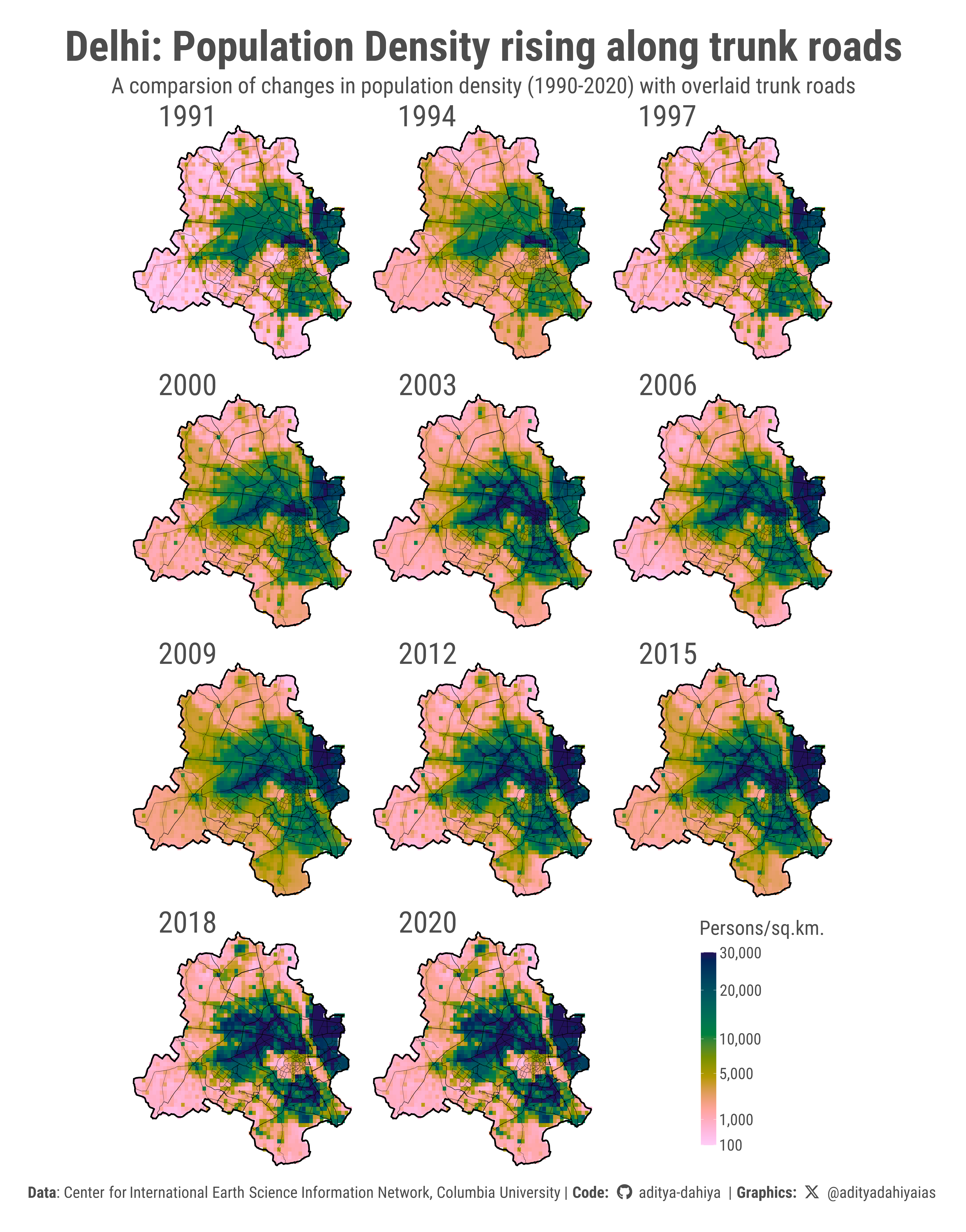
Figure 1: This graphic shows the population density of Delhi (India) compared from 1990 to 2020, on a transformed fill scale where darker colours represent more densely populated areas. Overlain on top are the major arterial roads of Delhi, taken from Open Street Maps data. An evident pattern is urban densification along major arterial roads, particularly towards north-west of Central Delhi, and especially along its Ring-Road.

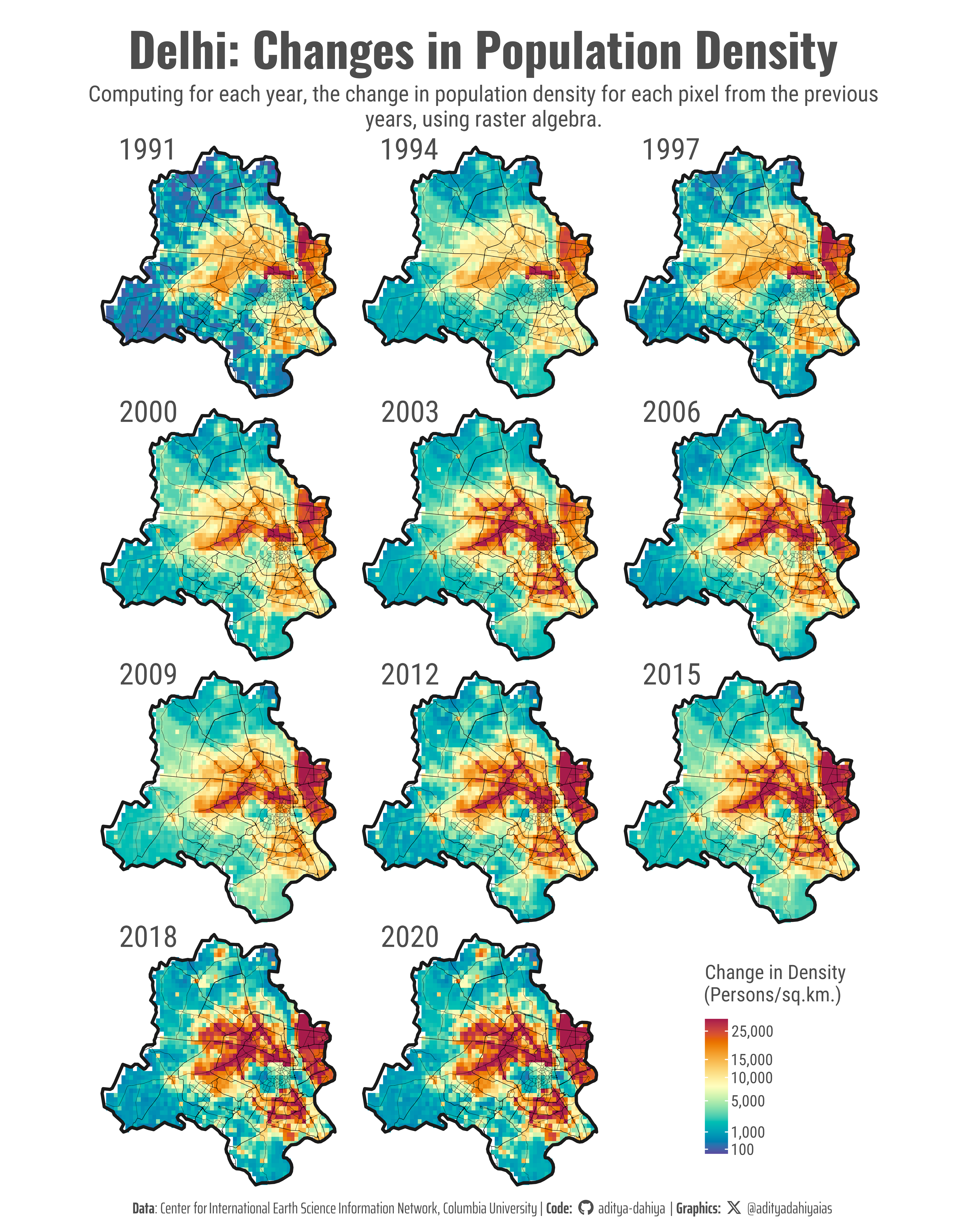
Plotting changes in population density over time

This code computes the difference between consecutive raster layers using map2() from the {purrr} package.

# Assuming delhi_rast_stack is a SpatRaster
years <- names(delhi_rast_stack) |> as.numeric()

# Compute differences between consecutive years
# {purrr}'s map2() function iterates over two vectors simultaneously.
rast_diff_list <- map2(
  
  # Removes the first element, keeping all years except the first 
  .x = years[-1], 
  
  # Removes the last element, keeping all years except the last
  .y = years[-length(years)], 
  
  # Each iteration computes the following
  .f = ~ {delhi_rast_stack[[as.character(.x)]] - delhi_rast_stack[[as.character(.y)]]}
)

# Convert the list to a raster stack
delhi_rast_diff <- rast(rast_diff_list)

# Rename layers to indicate change years (e.g., "Change_1991" for 1991-1990)
names(delhi_rast_diff) <- years[-1]
varnames(delhi_rast_diff) <- years[-1]

delhi_rast_diff

rm(years, rast_diff_list)

Plotting the differences (i.e. change in population density)

layers_to_keep <- which(
  names(delhi_rast_stack) %in% as.character(c(seq(1991, 2020, 3), 2020   ))
)


g <- ggplot() +
  geom_spatraster(
    data = delhi_rast_stack[[layers_to_keep]] |> 
      terra::mask(delhi_map, touches = FALSE)
  ) +
  geom_sf(
    data = delhi_map,
    linewidth = 2,
    fill = NA,
    colour = "grey10"
  ) +
  paletteer::scale_fill_paletteer_c(
    "grDevices::Spectral",
    direction = -1,
    na.value = "transparent",
    limits = c(-1e2, 3e4),
    breaks = c(-1e1, 0, 100, 1000, 5000, 10000, 15000, 25000),
    oob = scales::squish,
    trans = "sqrt",
    labels = label_number(big.mark = ",", accuracy = 1)
  ) +
  
  # Plotting Roads
  geom_sf(
    data = roads_delhi,
    mapping = aes(
      linewidth = width_var
    ),
    alpha = 1
  ) +
  scale_linewidth_manual(
    values = c(0.2, 0.2, 0.1, 0.05, 0.05)
  ) +
  facet_wrap(~lyr, ncol = 3) +
  coord_sf(
    clip = "off",
    expand = FALSE
  ) +
  guides(
    linewidth = "none"
  ) +
  labs(
    title = "Delhi: Changes in Population Density",
    subtitle = str_wrap("Computing for each year, the change in population density for each pixel from the previous years, using raster algebra.", 90),
    caption = plot_caption,
    fill = "Change in Density\n(Persons/sq.km.)"
  ) +
  theme_void(
    base_size = 80,
    base_family = "body_font"
  ) +
  theme(
    text = element_text(
      colour = text_hil
    ),
    strip.text = element_text(
      margin = margin(0,0,-20,0, "pt"),
      hjust = 0.1,
      size = 120
    ),
    panel.spacing.y = unit(0, "pt"),
    panel.spacing.x = unit(30, "pt"),
    legend.position = "inside",
    legend.position.inside = c(0.975, 0.03),
    legend.justification = c(1, 0),
    legend.text = element_text(
      margin = margin(0,0,0,5, "pt")
    ),
    legend.title = element_text(
      margin = margin(0,0,20,0, "pt"),
      lineheight = 0.3
    ),
    legend.key.height = unit(35, "pt"),
    legend.key.width = unit(30, "pt"),
    legend.ticks = element_line(
      linewidth = 0.7,
      colour = "white"
    ),
    panel.background = element_rect(
      fill = "transparent",
      colour = "transparent"
    ),
    plot.title = element_text(
      hjust = 0.5,
      margin = margin(40,0,5,0, "pt"),
      size = 190,
      colour = text_hil,
      face = "bold",
      family = "title_font"
    ),
    plot.subtitle = element_text(
      hjust = 0.5,
      margin = margin(5,0,5,0, "pt"),
      size = 90,
      colour = text_hil,
      lineheight = 0.3
    ),
    plot.caption = element_textbox(
      hjust = 0.5, 
      halign = 0.5,
      margin = margin(20,0,20,0, "pt"),
      colour = text_hil,
      family = "caption_font"
    )
  )

ggsave(
  plot = g,
  filename = here::here(
    "geocomputation", "images",
    "population_density_rasters_2.png"
  ),
  height = 1300 * 5.1,
  width = 1300 * 4,
  units = "px",
  bg = "white"
)

References

Liu, Luling, Xin Cao, Shijie Li, and Na Jie. 2024. “A 31-Year (19902020) Global Gridded Population Dataset Generated by Cluster Analysis and Statistical Learning.” Scientific Data 11 (1). https://doi.org/10.1038/s41597-024-02913-0.