Code
pacman::p_load(
  sf,
  terra,
  tidyterra,
  tidyverse,
  showtext,
  ggtext,
  fontawesome,
  geodata,
  ggmap
)Combining {sf}, {terra}, {tidyterra} and {osmdata} to make beautiful postal code maps
pacman::p_load(
sf,
terra,
tidyterra,
tidyverse,
showtext,
ggtext,
fontawesome,
geodata,
ggmap
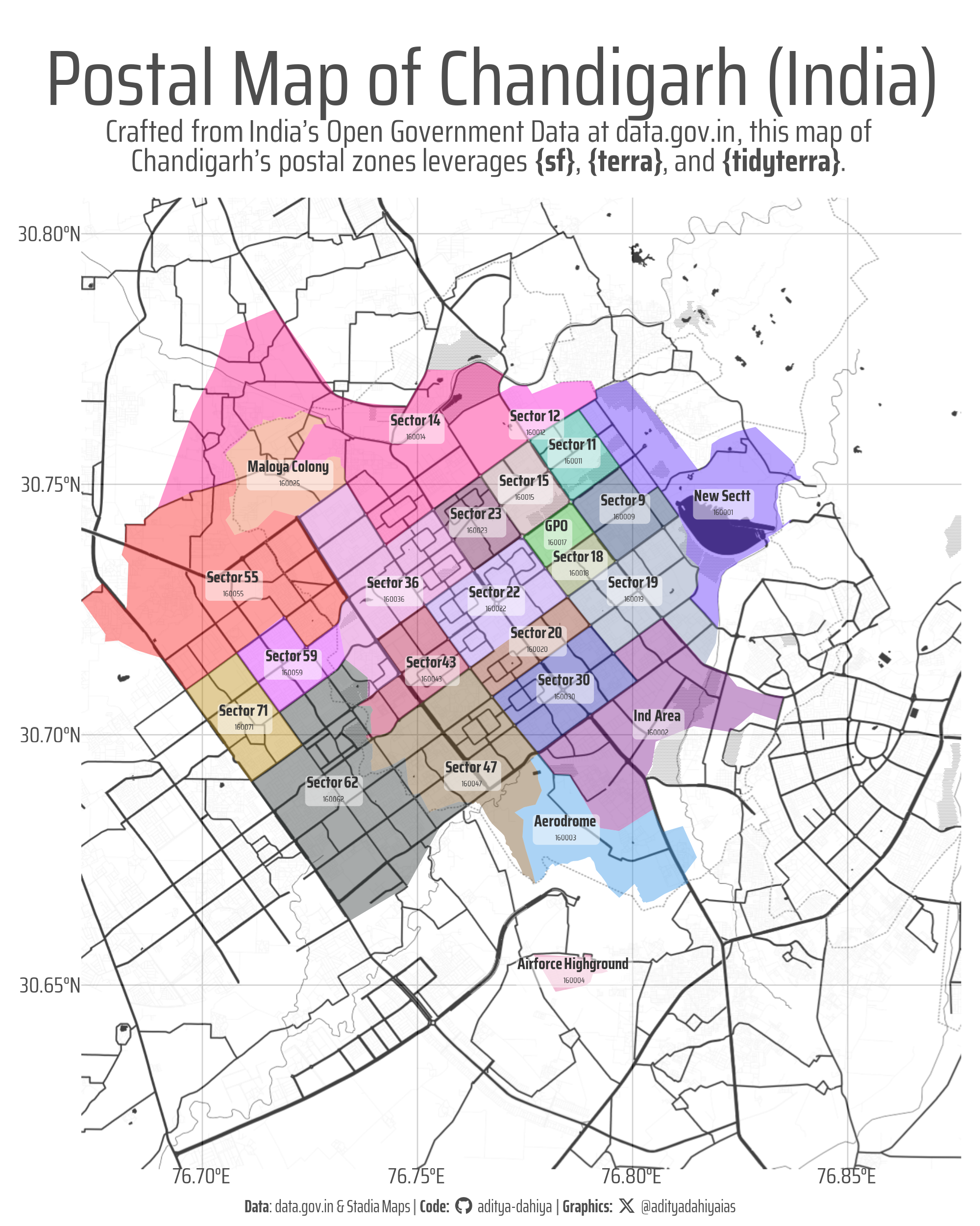
)The All India Pincode Boundary GeoJSON dataset, available on https://www.data.gov.in/catalog/all-india-pincode-boundary-geo-json, provides comprehensive geospatial information delineating postal code boundaries across India. This open data resource, published by the Government of India, includes GeoJSON files that map pincode regions with associated attributes such as pincode numbers, district names, and state names. The dataset is designed to facilitate applications in urban planning, logistics, demographic analysis, and geospatial research. Maintained under the Open Government Data (OGD) Platform India, it ensures accessibility and transparency, allowing developers, researchers, and policymakers to leverage accurate and standardized pincode-level geospatial data for various analytical and operational purposes.
india_pin_code <- read_sf(
  here::here(
    "data",
    "india_map",
    "All_India_pincode_Boundary-19312.geojson"
  )
) |>
  janitor::clean_names() |>
  st_transform("EPSG:4326") |>
  mutate(pincode = parse_number(pincode))

haryana_map <- read_sf(
  here::here(
    "data",
    "haryana_map",
    "HARYANA_DISTRICT_BDY.shp"
  )
) |>
  janitor::clean_names() |>
  mutate(
    district = str_replace_all(district, ">", "A"),
    district = str_replace_all(district, "\\|", "I"),
    district = str_to_title(district)
  ) |>
  st_transform("EPSG:4326")

haryana_outline <- read_sf(
  here::here(
    "data",
    "haryana_map",
    "HARYANA_STATE_BDY.shp"
  )
) |>
  janitor::clean_names() |>
  st_simplify(dTolerance = 1000) |>
  st_transform("EPSG:4326")

chandigarh_postal <- india_pin_code |>
  filter(pincode >= 160001 & pincode < 160100) |>
  mutate(
    label_name = str_remove_all(office_name, "SO"),
    label_name = str_remove_all(label_name, "Chandigarh"),
    label_name = paste(
      "<b>", label_name, "</b><br><span style='font-size:12pt'>",
      pincode,
      "</span>"
    )
  ) |>
  relocate(label_name)


# register_stadiamap("YOUR KEY HERE")
get_map_bbox <- chandigarh_postal |>
  st_bbox()
names(get_map_bbox) <- c("left", "bottom", "right", "top")

base_map <- get_stadiamap(
  bbox = get_map_bbox,
  zoom = 13,
  maptype = "stamen_toner_background"
) |>
  terra::rast()

# ggplot() +
#   geom_spatraster_rgb(data = base_map)

# Get post offices in Chandigarh
pacman::p_load(osmdata)

chandigarh_postoffices <- opq(bbox = st_bbox(chandigarh_postal)) |>
  add_osm_feature(
    key = "amenity",
    value = c("post_office", "post_box", "post_depot")
  ) |>
osmdata_sf()haryana_outline |>
ggplot() +
geom_sf()
haryana_map |>
st_drop_geometry() |>
select(district) |>
print(n = Inf)
india_pin_code |>
st_drop_geometry() |>
count(region, sort = T)
st_bbox(haryana_outline)
ggplot() +
geom_sf() +
geom_sf_text(
aes(label = str_wrap(office_name, 5)),
size = 2,
lineheight = 0.7
)# Visualization Parameters
bts = 12 # Base Text Size
sysfonts::font_add_google("Saira Condensed", "body_font")
sysfonts::font_add_google("Saira", "title_font")
sysfonts::font_add_google("Saira Extra Condensed", "caption_font")
showtext::showtext_auto()
# A base Colour
bg_col <- "white"
seecolor::print_color(bg_col)
# Colour for highlighted text
text_hil <- "grey30"
seecolor::print_color(text_hil)
# Colour for the text
text_col <- "grey20"
seecolor::print_color(text_col)
theme_set(
theme_minimal(
base_size = bts,
base_family = "body_font"
) +
theme(
text = element_text(
colour = "grey30",
lineheight = 0.3,
margin = margin(0,0,0,0, "pt")
),
plot.title = element_text(
hjust = 0.5
),
plot.subtitle = element_text(
hjust = 0.5
)
)
)
# Caption stuff for the plot
sysfonts::font_add(
family = "Font Awesome 6 Brands",
regular = here::here("docs", "Font Awesome 6 Brands-Regular-400.otf")
)
github <- ""
github_username <- "aditya-dahiya"
xtwitter <- ""
xtwitter_username <- "@adityadahiyaias"
social_caption_1 <- glue::glue("<span style='font-family:\"Font Awesome 6 Brands\";'>{github};</span> <span style='color: {text_hil}'>{github_username} </span>")
social_caption_2 <- glue::glue("<span style='font-family:\"Font Awesome 6 Brands\";'>{xtwitter};</span> <span style='color: {text_hil}'>{xtwitter_username}</span>")
plot_caption <- paste0(
"**Data**: data.gov.in & Stadia Maps",
" | **Code:** ",
social_caption_1,
" | **Graphics:** ",
social_caption_2
)
rm(github, github_username, xtwitter,
xtwitter_username, social_caption_1,
social_caption_2)This map of postal zones and post office boundaries in Chandigarh, India, was crafted using R and a suite of powerful packages for spatial data manipulation and visualization. The process started by loading key packages with pacman::p_load(), including sf for handling vector spatial data, terra for raster data support, tidyterra for integrating raster data with ggplot2, tidyverse for data wrangling, ggmap for fetching base maps, showtext for custom fonts, and ggtext for rich text labeling. I imported the All India Pincode Boundary GeoJSON data using read_sf() from the sf package, transformed it to the EPSG:4326 coordinate system with st_transform(), and filtered it to include only Chandigarh’s postal codes (160001 to 160099). A base map was retrieved from Stadia Maps via get_stadiamap(), using the bounding box of the Chandigarh postal data. The map was then built with ggplot2, layering the base map raster with geom_spatraster_rgb(), postal boundaries with geom_sf(), and post office labels with geom_richtext(). Custom fonts were applied using showtext, and the plot was polished with a minimal theme and saved as a high-resolution PNG using ggsave().
size_var = 2000
bts = size_var / 30

# nrow(chandigarh_postal)
# cols4all::c4a_gui()
# cols4all::c4a("poly.dark24")


g <- ggplot() +
  geom_spatraster_rgb(
    data = base_map,
    maxcell = Inf,
    alpha = 0.75
  ) +
  geom_sf(
    data = chandigarh_postal,
    mapping = aes(fill = office_name),
    colour = "transparent",
    linewidth = 2,
    alpha = 0.4
  ) +
  ggtext::geom_richtext(
    data = chandigarh_postal,
    mapping = aes(
      label = label_name,
      geometry = geometry
    ),
    fill = alpha("white", 0.5),
    colour = text_col,
    lineheight = 0,
    size = bts / 8,
    hjust = 0.5,
    vjust = 0.5,
    family = "body_font",
    stat = "sf_coordinates",
    label.size = NA,
    label.padding = unit(0.05, "lines")
  ) +
  # geom_sf(
  #   data = chandigarh_postoffices$osm_points,
  #   size = 5
  # ) +
  cols4all::scale_fill_discrete_c4a_cat("poly.dark24") +
  labs(
    x = NULL, y = NULL,
    title = "Postal Map of Chandigarh (India)",
    subtitle = "Crafted from India's Open Government Data at *data.gov.in*, this map of Chandigarh's postal zones leverages **{sf}**, **{terra}**, and **{tidyterra}**." |> str_wrap(80) |> str_replace_all("\n", "<br>"),
    caption = plot_caption
  ) +
  coord_sf(
    crs = "EPSG:3857",
    expand = FALSE
  ) +
  theme_minimal(
    base_size = bts,
    base_family = "body_font",
    base_line_size = bts / 140,
    base_rect_size = bts / 140
  ) +
  theme(

    # Plot / Overall
    plot.margin = margin(5,5,5,5, "pt"),
    plot.title.position = "plot",
    plot.caption.position = "plot",
    text = element_text(
      colour = text_hil,
      lineheight = 0.3,
      margin = margin(0,0,0,0, "pt")
    ),

    # Plot Title, Subtitle and Caption
    plot.title = element_text(
      margin = margin(20,0,0,0, "pt"),
      hjust = 0.5,
      size = bts * 1.8
    ),
    plot.subtitle = element_textbox(
      margin = margin(0,0,10,0, "pt"),
      hjust = 0.5,
      halign = 0.5,
      size = bts / 1.4
    ),
    plot.caption = element_textbox(
      margin = margin(5,0,0,0, "pt"),
      halign = 0.5,
      hjust = 0.5,
      size = 0.4 * bts,
      family = "caption_font"
    ),
    axis.text.x = element_text(
      size = bts / 2,
      margin = margin(-0.5,0,0,0, "pt")
    ),
    axis.text.y = element_text(
      size = bts / 2,
      margin = margin(0,-0.5,0,0, "pt")
    ),
    axis.ticks.length = unit(0, "pt"),
    axis.ticks = element_blank(),

    # Legend
    legend.position = "none",

    # Panel
    panel.grid = element_line(
      linewidth = 0.3,
      colour = "grey30"
    )
  )


ggsave(
  plot = g,
  filename = here::here("geocomputation", "images",
                        "postal_code_maps_1.png"),
  width = size_var,
  height = (5/4) * size_var,
  units = "px",
  bg = bg_col
)