Exploring the package {rnaturalearth} in R

Various types of maps and geographic data available with {rnaturalearth}

Introduction

# Data wrangling & visualization
library(tidyverse)  # Data manipulation & visualization

# Spatial data handling
library(sf)         # Import, export, and manipulate vector data
library(terra)      # Import, export, and manipulate raster data

# ggplot2 extensions
library(tidyterra)  # Helper functions for using terra with ggplot2

# Final plot tools
library(scales)               # Nice Scales for ggplot2
library(fontawesome)          # Icons display in ggplot2
library(ggtext)               # Markdown text in ggplot2
library(showtext)             # Display fonts in ggplot2
library(patchwork)            # Composing Plots

# Package to explore
library(rnaturalearth)        # Open Source Geographic data

bts = 12 # Base Text Size
sysfonts::font_add_google("Roboto Condensed", "body_font")
sysfonts::font_add_google("Oswald", "title_font")
showtext::showtext_auto()
# A base Colour
bg_col <- "white"
seecolor::print_color(bg_col)

# Colour for highlighted text
text_hil <- "grey30"
seecolor::print_color(text_hil)

# Colour for the text
text_col <- "grey20"
seecolor::print_color(text_col)

theme_set(
  theme_minimal(
    base_size = bts,
    base_family = "body_font"
  ) +
    theme(
      text = element_text(
        colour = "grey30",
        lineheight = 0.3,
        margin = margin(0,0,0,0, "pt")
      ),
      plot.title = element_text(
        hjust = 0.5
      ),
      plot.subtitle = element_text(
        hjust = 0.5
      )
    )
)

# Caption stuff for the plot
sysfonts::font_add(
  family = "Font Awesome 6 Brands",
  regular = here::here("docs", "Font Awesome 6 Brands-Regular-400.otf")
)
github <- "&#xf09b"
github_username <- "aditya-dahiya"
xtwitter <- "&#xe61b"
xtwitter_username <- "@adityadahiyaias"
social_caption_1 <- glue::glue("<span style='font-family:\"Font Awesome 6 Brands\";'>{github};</span> <span style='color: {text_hil}'>{github_username}  </span>")
social_caption_2 <- glue::glue("<span style='font-family:\"Font Awesome 6 Brands\";'>{xtwitter};</span> <span style='color: {text_hil}'>{xtwitter_username}</span>")
plot_caption <- paste0(
  "**Tools**: {rnaturalearth}  ",
  "  |  **Code:** ", 
  social_caption_1, 
  " |  **Graphics:** ", 
  social_caption_2
  )
rm(github, github_username, xtwitter, 
   xtwitter_username, social_caption_1, 
   social_caption_2)

Basic plot of World Map

world1 <- rnaturalearth::ne_countries(
  scale = "medium",
  returnclass = "sf"
)

g <- ggplot(world1) +
  geom_sf(
    fill = alpha("grey", 0.8), colour = "grey30",
    linewidth = 0.1
  ) +
  coord_sf(
    crs = "ESRI:54030"
  ) +
  labs(
    title = "Basic world map with ne_countries()"
  ) +
  theme(
    plot.title = element_textbox(
      hjust = 0.5, 
      halign = 0.5
    ),
    panel.grid = element_line(
      linewidth = 0.05, 
      colour = "grey20",
      linetype = 2
    )
  )

ggsave(
  plot = g,
  filename = here::here(
    "geocomputation", "images",
     "rnaturalearth_package_1.png"
  ),
  height = 500,
  width = 800,
  units = "px"
)

Figure 1: Basic World map with ne_countries()

World Coastline Map

world1 <- rnaturalearth::ne_coastline(
  scale = "medium",
  returnclass = "sf"
)

g <- ggplot(world1) +
  geom_sf(
    fill = alpha("grey", 0.8), colour = "grey30",
    linewidth = 0.1
  ) +
  coord_sf(
    crs = "ESRI:54030"
  ) +
  labs(
    title = "Basic Coastline map with ne_coastline()",
    subtitle = "Multi-linestring class of {sf} objects"
  ) +
  theme(
    plot.title = element_textbox(
      hjust = 0.5, 
      halign = 0.5
    ),
    panel.grid = element_line(
      linewidth = 0.05, 
      colour = "grey20",
      linetype = 2
    )
  )

ggsave(
  plot = g,
  filename = here::here(
    "geocomputation", "images",
     "rnaturalearth_package_2.png"
  ),
  height = 500,
  width = 800,
  units = "px"
)

Oceans map with ne_download

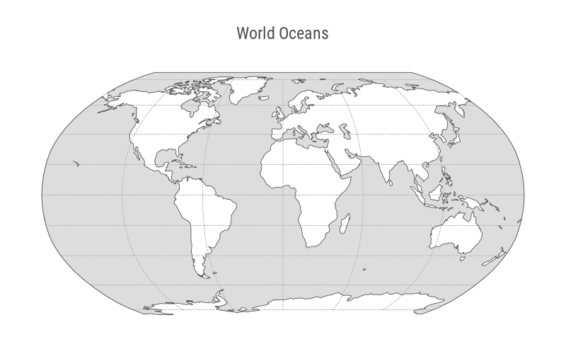
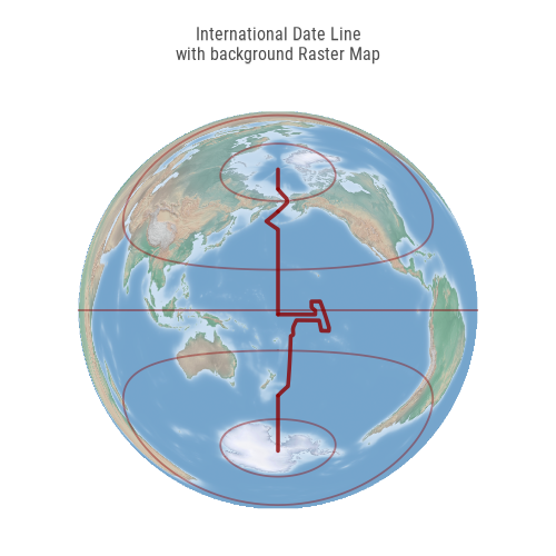
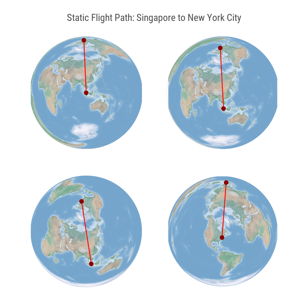
Entire world water bodies as 1 (or 2, for Caspian Sea) multipolygons. Useful for plotting flight paths, when we don’t want oceans to be transparent in Azimuthal Equal Area projections.

# Link: https://www.naturalearthdata.com/http//www.naturalearthdata.com/download/110m/physical/ne_110m_ocean.zip

world_oceans <- ne_download(
  scale = 50,
  type = "ocean",
  category = "physical",
  returnclass = "sf"
)

g <- ggplot(world_oceans) +
  geom_sf(
    fill = alpha("grey", 0.5),
    linewidth = 0.1
  ) +
  coord_sf(crs = "ESRI:54030") +
  labs(
    title = "World Oceans"
  ) +
  theme(
    plot.title = element_textbox(
      hjust = 0.5, 
      halign = 0.5,
      size = 18
    ),
    panel.grid = element_line(
      linewidth = 0.05, 
      colour = "grey20",
      linetype = 2
    )
  )

ggsave(
  plot = g,
  filename = here::here(
    "geocomputation", "images",
     "rnaturalearth_package_3.png"
  ),
  height = 500,
  width = 800,
  units = "px"
)

Geographic lines with ne_download()

# https://www.naturalearthdata.com/http//www.naturalearthdata.com/download/50m/physical/ne_50m_geographic_lines.zip

world_map <- ne_countries(
  scale = 110,
  returnclass = "sf"
) |> 
  select(name, geometry)

world_lines <- ne_download(
  scale = 50,
  type = "geographic_lines",
  returnclass = "sf",
  category = "physical"
) |> 
  select(name) |> 
  mutate(
    high_var = name == "International Date Line"
  )

g <- ggplot() +
  geom_sf(
    data = world_map,
    fill = alpha("grey", 0.5),
    linewidth = 0.1
  ) +
  geom_sf(
    data = world_lines,
    mapping = aes(
      linewidth = high_var,
      alpha = high_var
    ),
    colour = "darkred",
    linetype = 1,
    lineend = "round"
  ) +
  scale_alpha_manual(values = c(0.4, 0.8)) +
  scale_linewidth_manual(values = c(0.2, 0.4)) +
  coord_sf(
    crs = paste0(
        "+proj=laea +x_0=0 +y_0=0 +lon_0=", 
        180, 
        " +lat_0=", 
        0)
    ) +
  labs(
    title = "International Date Line"
  ) +
  theme(
    plot.title = element_textbox(
      hjust = 0.5, 
      halign = 0.5,
      size = 18
    ),
    panel.grid = element_blank(),
    legend.position = "none"
  )

ggsave(
  plot = g,
  filename = here::here(
    "geocomputation", "images",
     "rnaturalearth_package_4.png"
  ),
  height = 500,
  width = 500,
  units = "px"
)

Raster Maps for the World with ne_download()

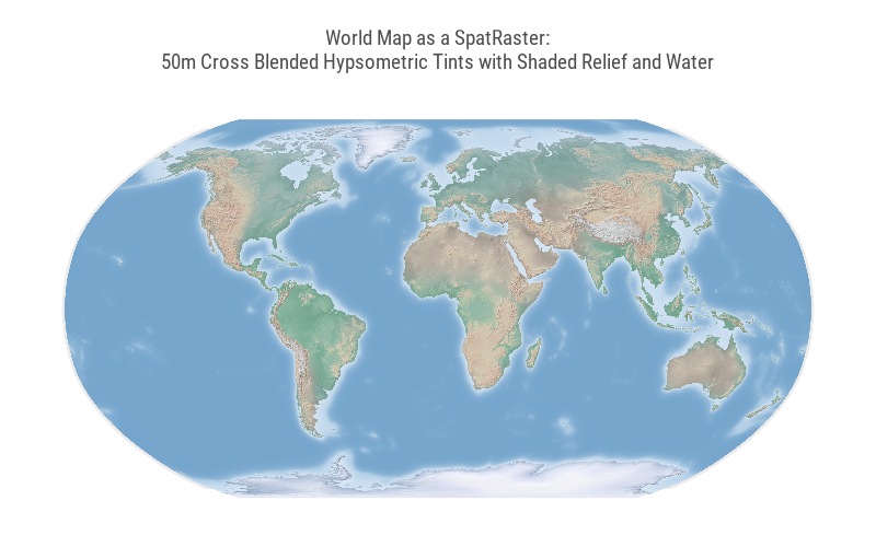
In this case, we are downloading the 50m Cross Blended Hypsometric Tints with Shaded Relief dataset, which combines elevation-based color shading with hillshade effects to enhance terrain visualization. This dataset is ideal for creating aesthetically pleasing and informative background maps in ggplot2 with tidyterra, providing a smooth, global-scale representation of landforms.

# Link to data: https://www.naturalearthdata.com/downloads/50m-raster-data/50m-cross-blend-hypso

# https://www.naturalearthdata.com/http//www.naturalearthdata.com/download/50m/raster/HYP_50M_SR.zip

# https://www.naturalearthdata.com/http//www.naturalearthdata.com/download/50m/raster/HYP_50M_SR_W.zip

world_cbhsr_rast <- ne_download(
  scale = 50,
  type = "HYP_50M_SR_W",
  category = "raster"
)

temp_rast <- world_cbhsr_rast |> 
  aggregate(fact = 2) |> 
  project("ESRI:54030")
g <- ggplot() +
  geom_spatraster_rgb(
    data = temp_rast,
    maxcell = 5e6
  ) +
  labs(
    title = "World Map as a SpatRaster:\n50m Cross Blended Hypsometric Tints with Shaded Relief and Water"
  ) 

ggsave(
  plot = g,
  filename = here::here(
    "geocomputation", "images",
     "rnaturalearth_package_5.png"
  ),
  height = 500,
  width = 800,
  units = "px"
)

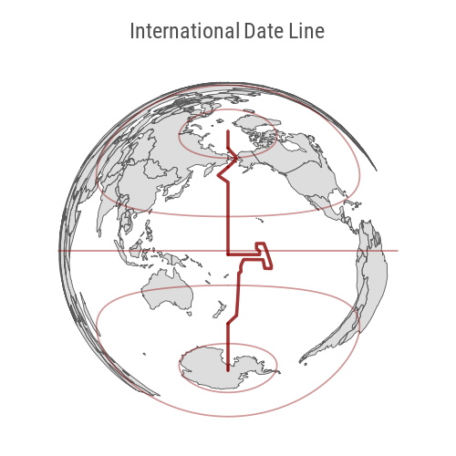
Plotting International Date Line with Raster Map

Changing the CRS to Azimuthal Equal Area Projection around Equator and IDL cross-point.

temp_crs <- paste0(
  "+proj=laea +x_0=0 +y_0=0 +lon_0=", 
  180,          # Longitude
  " +lat_0=", 
  0             # Latitude
)

temp_rast <- world_cbhsr_rast |> 
  terra::aggregate(fact = 10) |> 
  terra::project(temp_crs)

g <- ggplot() +
  geom_spatraster_rgb(
    data = temp_rast
  ) +
  geom_sf(
    data = world_lines,
    mapping = aes(
      linewidth = high_var,
      alpha = high_var
    ),
    colour = "darkred",
    linetype = 1,
    lineend = "round"
  ) +
  scale_alpha_manual(values = c(0.4, 0.8)) +
  scale_linewidth_manual(values = c(0.2, 0.4)) +
  coord_sf(
    crs = 
    ) +
  labs(
    title = "International Date Line\nwith background Raster Map"
  ) +
  theme(
    plot.title = element_text(
      hjust = 0.5, size = 12
    ),
    panel.grid = element_blank(),
    legend.position = "none"
  )


ggsave(
  plot = g,
  filename = here::here(
    "geocomputation", "images",
     "rnaturalearth_package_6.png"
  ),
  height = 500,
  width = 500,
  units = "px"
)

Flight path from one place to another

# Basic World Maps (repeat of previous code)
world_map <- ne_countries(
  scale = 110,
  returnclass = "sf"
) |> 
  select(name, geometry)

world_lines <- ne_download(
  scale = 50,
  type = "geographic_lines",
  returnclass = "sf",
  category = "physical"
) |> 
  select(name) |> 
  mutate(
    high_var = name == "International Date Line"
  )

world_oceans <- ne_download(
  scale = 50,
  type = "ocean",
  category = "physical",
  returnclass = "sf"
) 

# Number of flight path points to treat as intermediate between 
# Singapore and New York City
num_points <- 20

flight1 <- tibble::tibble(
  name = c("Singapore Changi Airport", 
           "New York JFK Airport"),
  longitude = c(103.994003, -73.7781),
  latitude = c(1.364420, 40.6413)
)

flight2 <- flight1 |> 
  st_as_sf(
    coords = c("longitude", "latitude"),
    crs = "EPSG:4326"
  )

flight_path <- geosphere::gcIntermediate(
  p1 = c(flight1$longitude[1], flight1$latitude[1]),
  p2 = c(flight1$longitude[2], flight1$latitude[2]),
  n = num_points,
  addStartEnd = TRUE
) |> 
  as_tibble()

flight_path_sf <- flight_path |>
  st_as_sf(
    coords = c("lon", "lat"),
    crs = "EPSG:4326"
  ) |> 
  st_combine() |> 
  st_cast("LINESTRING")


# Points to plot
plot_points <- c(1, num_points %/% 3, 
                 2*num_points %/% 3, num_points)

for (i in plot_points){
  
  temp_crs <- paste0(
    "+proj=laea +x_0=0 +y_0=0 +lon_0=", 
    flight_path$lon[i],          # Longitude
    " +lat_0=", 
    flight_path$lat[i]            # Latitude
  )
  
  temp_rast <- world_cbhsr_rast |> 
    terra::aggregate(fact = 10) |> 
    terra::project(temp_crs)
  
paste0("g", i) |> 
  assign(
    ggplot() +
      geom_spatraster_rgb(
        data = temp_rast
      ) +
      # geom_sf(
      #   data = world_map,
      #   fill = "#e0ca22",
      #   colour = NA,
      #   linewidth = 0.01
      # ) +
      # geom_sf(
      #   data = world_oceans,
      #   fill = "skyblue",
      #   colour = NA
      # ) +
      geom_sf(
        data = flight_path_sf, 
        colour = "red",
        linewidth = 0.3
        ) +
      geom_sf(
        data = flight2,
        size = 1,
        colour = "darkred"
      ) +
      coord_sf(
        crs = temp_crs
      ) +
      theme(
        plot.title = element_textbox(
          hjust = 0.5, 
          halign = 0.5
        ),
        panel.grid = element_line(
          linewidth = 0.05, 
          colour = "grey80",
          linetype = 1
        )
      )
  )
  
}

g <- g1 + g6 + g12 + g20 +
  plot_annotation(
    title = "Static Flight Path: Singapore to New York City",
    theme = theme(
      plot.title = element_text(
        size = 2 * 12,
        margin = margin(5,0,0,0, "pt")
      )
    )
  )

ggsave(
  plot = g,
  filename = here::here(
    "geocomputation", "images",
     "rnaturalearth_package_7.png"
  ),
  height = 1000,
  width = 1000,
  units = "px"
)

Get an animation of flight path

world_agg_rast <- world_cbhsr_rast |> 
    terra::aggregate(fact = 10)


# Number of flight path points to treat as intermediate between 
# Singapore and New York City
num_points <- 20

flight1 <- tibble::tibble(
  name = c("Singapore Changi Airport", 
           "New York JFK Airport"),
  longitude = c(103.994003, -73.7781),
  latitude = c(1.364420, 40.6413)
)

flight2 <- flight1 |> 
  st_as_sf(
    coords = c("longitude", "latitude"),
    crs = "EPSG:4326"
  )

flight_path <- geosphere::gcIntermediate(
  p1 = c(flight1$longitude[1], flight1$latitude[1]),
  p2 = c(flight1$longitude[2], flight1$latitude[2]),
  n = num_points,
  addStartEnd = TRUE
) |> 
  as_tibble()

flight_path_sf <- flight_path |>
  st_as_sf(
    coords = c("lon", "lat"),
    crs = "EPSG:4326"
  ) |> 
  st_combine() |> 
  st_cast("LINESTRING")

library(magick)
library(animation)

i = 10

animation::saveGIF(
  
  expr = for (i in 1:nrow(flight_path)) {
    temp_crs <- paste0(
      "+proj=laea +x_0=0 +y_0=0 +lon_0=", 
      flight_path$lon[i],          # Longitude
      " +lat_0=", 
      flight_path$lat[i]            # Latitude
    )
  
    temp_rast <- world_agg_rast |> 
      terra::project(temp_crs)
  
    ggplot() +
      geom_spatraster_rgb(
        data = temp_rast,
        maxcell = 5e+4
      ) +
      geom_sf(
        data = flight_path_sf, 
        colour = "red",
        linewidth = 0.3
        ) +
      geom_sf(
        data = flight2,
        size = 0.6,
        colour = "darkred"
      ) +
      geom_sf(
        data = flight_path |> 
                  slice(i) |> 
                  st_as_sf(coords = c("lon", "lat"),
                           crs = "EPSG:4326"),
        size = 1,
        colour = "grey20"
      ) +
      coord_sf(
        crs = temp_crs
      )
  },
  movie.name = here::here(
    "geocomputation", "images",
    "rnaturalearth_package_1.gif"
  ),
  ani.height = 500,
  ani.width = 500,
  ani.loop = TRUE,
  interval = 1
)

ne_states() with India

# Get border map of Uttarakhand
uk_state = ne_states(country = "India", returnclass = "sf") |> 
  select(iso_3166_2, name, geometry) |> 
  filter(name == "Uttarakhand")


# Get Rivers of Uttarakhand
# https://www.naturalearthdata.com/downloads/50m-physical-vectors/
# https://www.naturalearthdata.com/http//www.naturalearthdata.com/download/50m/physical/ne_50m_rivers_lake_centerlines.zip
uk_rivers <- ne_download(
  scale = 10,
  type = "rivers_lake_centerlines",
  category = "physical",
  returnclass = "sf"
) |> 
  st_intersection(uk_state)

# Get Lakes of Uttarakhand
# https://www.naturalearthdata.com/http//www.naturalearthdata.com/download/50m/physical/ne_50m_lakes.zip
uk_lakes <- ne_download(
  scale = 50,
  type = "lakes",
  category = "physical",
  returnclass = "sf"
)

uk_lakes |> 
  ggplot() +
  geom_sf()

uk_rivers |> 
  ggplot() +
  geom_sf()

uk_state |> 
  ggplot() +
  geom_sf()