Showing elevation in Maps (2) : {whitebox} & {terra}

Exploring {whitebox} & {terra} for shaded relief maps with {ggplot2} and {tidyterra}

Maps

Geocomputation

{whitebox}

{terra}

Author

Aditya Dahiya

Published

February 3, 2025

In this project, we apply hillshade techniques to visualize the topography of Sikkim, India, using digital elevation models (DEMs). Hillshading, a method that simulates shadows cast by terrain, enhances the three-dimensional appearance of elevation data, making it valuable for geospatial analysis through resources like the USGS. This work follows Dr. Dominic Royé’s guide on generating hillshade effects using R, as outlined in Dominic Royé’s Blog.

We employ R’s geospatial packages, including terra for raster processing, rayshader for 3D rendering, and elevatr for retrieving elevation data from sources such as NASA’s SRTM. These techniques effectively highlight Sikkim’s complex Himalayan terrain, essential for environmental monitoring, disaster risk assessment, and ecological studies. The approach can also be extended to land-use planning and hydrological modeling.

Code

# Data wrangling & visualization
library(tidyverse)  # Data manipulation & visualization

# Spatial data handling
library(sf)         # Import, export, and manipulate vector data
library(terra)      # Import, export, and manipulate raster data
library(elevatr)    # Access elevation data from APIs

# Geospatial processing
library(whitebox)   # WhiteboxTools for geospatial analysis

# ggplot2 extensions
library(tidyterra)  # Helper functions for using terra with ggplot2
library(ggnewscale) # Support multiple scales in ggplot2
library(ggblend)    # Enable color blending in ggplot2

# Final plot tools
library(scales)               # Nice Scales for ggplot2
library(fontawesome)          # Icons display in ggplot2
library(ggtext)               # Markdown text in ggplot2
library(showtext)             # Display fonts in ggplot2
library(colorspace)           # Lighten and Darken colours
library(patchwork)            # Composing Plots

bts = 18 # Base Text Size
sysfonts::font_add_google("Roboto Condensed", "body_font")
sysfonts::font_add_google("Oswald", "title_font")
showtext::showtext_auto()
theme_set(
  theme_minimal(
    base_size = bts,
    base_family = "body_font"
  ) +
    theme(
      text = element_text(
        colour = "grey30",
        lineheight = 0.3,
        margin = margin(0,0,0,0, "pt")
      ),
      plot.title = element_text(
        hjust = 0.5
      ),
      plot.subtitle = element_text(
        hjust = 0.5
      )
    )
)

# Some basic caption stuff
# A base Colour
bg_col <- "white"
seecolor::print_color(bg_col)

# Colour for highlighted text
text_hil <- "grey30"
seecolor::print_color(text_hil)

# Colour for the text
text_col <- "grey20"
seecolor::print_color(text_col)


# Caption stuff for the plot
sysfonts::font_add(
  family = "Font Awesome 6 Brands",
  regular = here::here("docs", "Font Awesome 6 Brands-Regular-400.otf")
)
github <- "&#xf09b"
github_username <- "aditya-dahiya"
xtwitter <- "&#xe61b"
xtwitter_username <- "@adityadahiyaias"
social_caption_1 <- glue::glue("<span style='font-family:\"Font Awesome 6 Brands\";'>{github};</span> <span style='color: {text_hil}'>{github_username}  </span>")
social_caption_2 <- glue::glue("<span style='font-family:\"Font Awesome 6 Brands\";'>{xtwitter};</span> <span style='color: {text_hil}'>{xtwitter_username}</span>")
plot_caption <- paste0(
  "**Tools**: {elevatr} {terra} {tidyterra} in *#rstats* ",
  "  |  **Code:** ", 
  social_caption_1, 
  " |  **Graphics:** ", 
  social_caption_2
  )
rm(github, github_username, xtwitter, 
   xtwitter_username, social_caption_1, 
   social_caption_2)

Trying the technique for Sikkim (India)

The following code extracts and visualizes geographical features of Sikkim using OpenStreetMap data. The osmdata package is used to fetch water bodies (lakes, ponds) and road networks within the Sikkim state boundary. First, the administrative boundary of Sikkim is read from a shapefile using sf and transformed to EPSG:4326. Then, opq() queries OpenStreetMap for water features (natural = water) and roads (highway key). The top 20 largest lakes are selected based on area, and major roads are filtered. Finally, ggplot2 is used to plot the Sikkim boundary along with lakes.

Code

library(osmdata)        # Fetching lakes data

# Get sikkim administrative boundary data
sikkim_vec <- read_sf(
  here::here(
    "data", "india_map",
    "India_State_Boundary.shp"
  )
) |> 
  filter(State_Name == "Sikkim") |> 
  st_transform("EPSG:4326")

# Add lakes, ponds and water bodies
sikkim_lakes_raw <- opq(bbox = st_bbox(sikkim_vec)) |>
  add_osm_feature(
    key = "natural",
    value = c("water")
  ) |>
  osmdata_sf()

sikkim_lakes <- bind_rows(
  sikkim_lakes_raw$osm_polygons,
  sikkim_lakes_raw$osm_multipolygons
) |> 
  select(osm_id, geometry) |> 
  st_crop(sikkim_vec) |> 
  mutate(
    area = st_area(geometry)
  ) |>
  slice_max(order_by = area, n = 20)

# Getting roads
sikkim_roads_raw <- opq(bbox = st_bbox(sikkim_vec)) |>
  add_osm_feature(
    key = "highway", 
    value = c("motorway", "trunk",
              "primary", "secondary")
  ) |>
  osmdata_sf()
object.size(sikkim_roads_raw) |> print(units = "Mb")

levels_roads <- c("secondary", "primary", "trunk")

sikkim_roads <- sikkim_roads_raw$osm_lines |> 
  select(osm_id, highway, geometry) |> 
  mutate(highway = fct(highway, levels = levels_roads)) |> 
  st_intersection(sikkim_vec)

ggplot() +
  geom_sf(data = sikkim_vec, fill = NA) +
  geom_sf(data = sikkim_lakes)

Elevation Raster Map

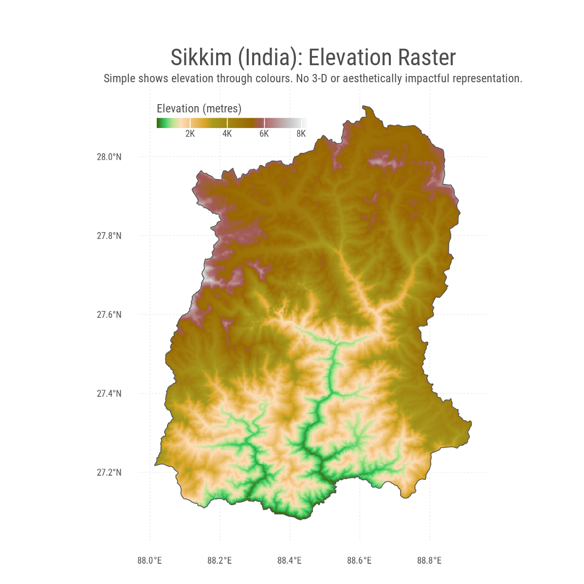
The following code visualizes the elevation data of Sikkim, India using the {ggplot2} and {terra} packages. It first plots the vector boundary of Sikkim using {sf} and then retrieves a Digital Elevation Model (DEM) using {elevatr}’s get_elev_raster(). The raster data is then converted to a {terra} object, cropped, and masked to match the Sikkim boundary. Finally, a ggplot2 map is created using geom_spatraster() to visualize elevation with a hypsometric color scale.

Code

# Test plot the sf object: a vector
ggplot(sikkim_vec) +
  geom_sf(fill = NA) +
  labs(title = "Sikkim (India)")

# Get DEM: Digital Elevation Model of Sikkim from {elevatr}
sikkim_rast <- elevatr::get_elev_raster(
  locations = sikkim_vec,
  z = 9
) |> 
  terra::rast() |> 
  terra::crop(sikkim_vec) |> 
  terra::mask(sikkim_vec)

g1 <- ggplot() +
  geom_spatraster(data = sikkim_rast) +
  geom_sf(data = sikkim_vec, fill = NA) +
  scale_fill_hypso_c(
    labels = scales::label_number(
      scale_cut = cut_short_scale()
    )
  ) +
  labs(
    title = "Sikkim (India): Elevation Raster",
    subtitle = "Simple shows elevation through colours. No 3-D or aesthetically impactful representation.",
    fill = "Elevation (metres)"
  ) +
  theme(
    legend.position = "inside",
    legend.position.inside = c(0,1),
    legend.justification = c(0,1),
    legend.key.height = unit(5, "pt"),
    legend.key.width = unit(15, "pt"),
    legend.title.position = "top",
    legend.direction = "horizontal",
    plot.title = element_text(
        size = bts * 2,
        margin = margin(15,0,2,0, "pt")
      ),
    plot.subtitle = element_text(
        size = bts,
        margin = margin(0,0,0,0, "pt")
      ),
    panel.grid = element_line(
        linewidth = 0.2,
        linetype = 3
    ),
    legend.title = element_text(
      margin = margin(0,0,2,0, "pt")
    ),
    legend.text = element_text(
      margin = margin(1,0,0,0, "pt")
    )
  )

ggsave(
  plot = g1,
  filename = here::here(
    "geocomputation", "images",
    "whitebox_terra_1.png"
  ),
  height = 1200,
  width = 1200,
  units = "px"
)

Grayscale Hillshade with Terrain Data

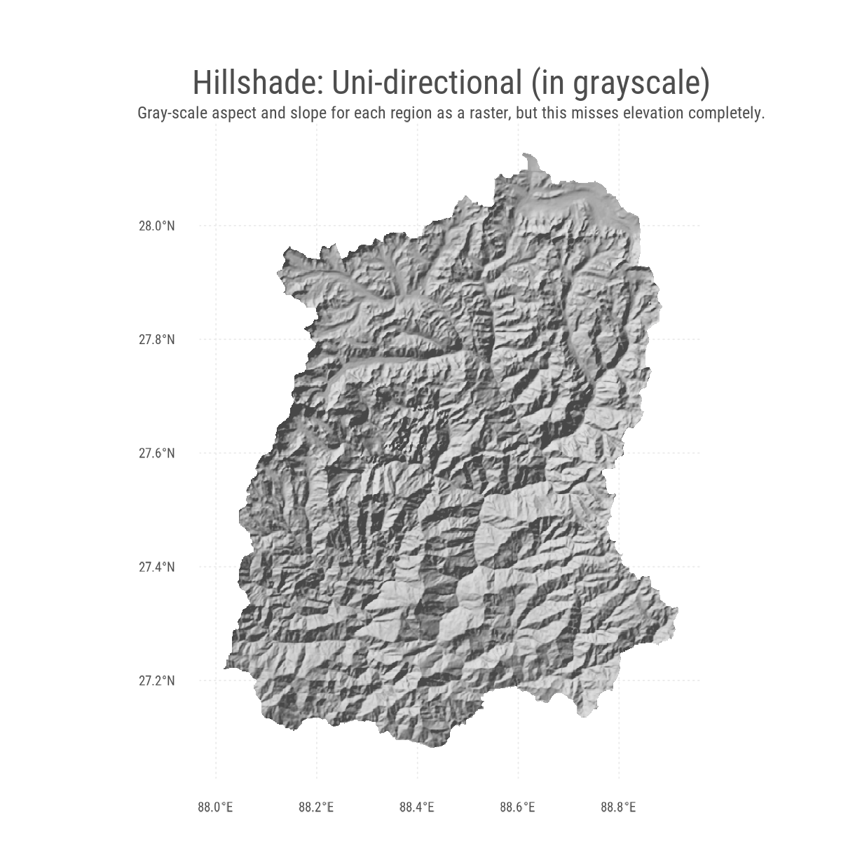
The following code demonstrates how to create a hillshade effect using the terra package for terrain analysis and ggplot2 for visualization. First, it calculates the slope and aspect of a raster dataset, representing terrain elevation. The terra::terrain() function is utilized to estimate both the slope and aspect in radians. Using a specified sun angle and direction, the hillshade effect is generated with the shade() function, providing a grayscale representation of the terrain. Finally, the hillshade is visualized with ggplot2, employing the geom_spatraster() function from the tidyterra package and a grayscale palette from the paletteer package. The plot is saved using ggsave() from the here package for organized file paths.

Code

# Estimate the Slope of the terrain using terra::terrain
slope1 <- terrain(sikkim_rast, v = "slope", unit = "radians")
# Estimate the Aspect or Orientation using terra::terrain
aspect1 <- terrain(sikkim_rast, v = "aspect", unit = "radians")

# With a certain Sun-Angle and Sun-Direction
sunangle = 30
sundirection = 315

# Calculate the hillshade effect with a certain degree of elevation
sikkim_shade_single <- shade(
  slope = slope1, 
  aspect = aspect1,
  angle = sunangle,
  direction = sundirection,
  normalize = TRUE
)

# Final Hill-shade Plot
g2 <- ggplot() +
  geom_spatraster(
    data = sikkim_shade_single
  ) +
  paletteer::scale_fill_paletteer_c(
    "grDevices::Light Grays",
    na.value = "transparent",
    direction = 1
  ) +
  labs(
    title = "Hillshade: Uni-directional (in grayscale)",
    subtitle = "Gray-scale aspect and slope for each region as a raster, but this misses elevation completely.",
    fill = "Elevation (metres)"
  ) +
  theme(
    legend.position = "none",
    plot.title = element_text(
        size = bts * 2,
        margin = margin(15,0,2,0, "pt")
      ),
    plot.subtitle = element_text(
        size = bts,
        margin = margin(0,0,0,0, "pt")
      ),
    panel.grid = element_line(
        linewidth = 0.2,
        linetype = 3
    ),
    legend.title = element_text(
      margin = margin(0,0,2,0, "pt")
    ),
    legend.text = element_text(
      margin = margin(1,0,0,0, "pt")
    )
  )

ggsave(
  plot = g2,
  filename = here::here(
    "geocomputation", "images",
    "whitebox_terra_2.png"
  ),
  height = 1200,
  width = 1200,
  units = "px"
)

Uni-directional Shadow: with a Coloured raster map

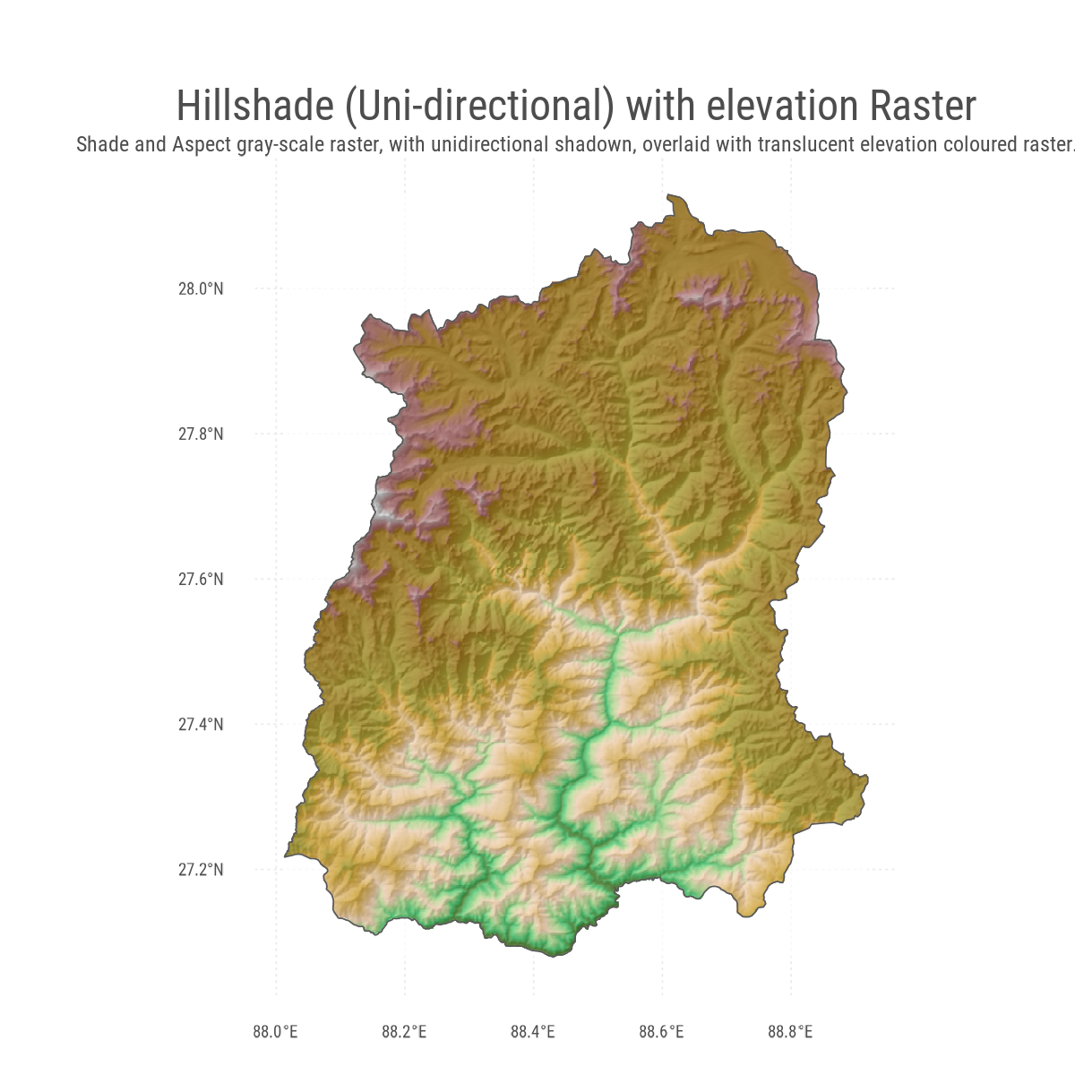
The following code generates a map overlaying a hillshade raster with an elevation raster for Sikkim. The hillshade raster, stored in sikkim_shade_single, is plotted first using geom_spatraster() from the terra package. It is styled using a grayscale palette from paletteer::scale_fill_paletteer_c(). A new fill scale is introduced with ggnewscale::new_scale_fill() before overlaying the elevation raster, sikkim_rast, with scale_fill_hypso_c() for elevation-based coloring. The outer boundary of Sikkim is added using geom_sf().

Code

g3 <- ggplot() +
  
  # The shadows part of the raster map
  geom_spatraster(
    data = sikkim_shade_single
  ) +
  paletteer::scale_fill_paletteer_c(
    "grDevices::Light Grays",
    na.value = "transparent",
    direction = 1
  ) +
  
  # New fill scale
  ggnewscale::new_scale_fill() +
  
  # The elevation digital raster
  geom_spatraster(
    data = sikkim_rast,
    alpha = 0.7
  ) +
  scale_fill_hypso_c() +
  
  # Outer boundary map of Sikkim
  geom_sf(
    data = sikkim_vec,
    fill = NA
  ) +
  
  labs(
    title = "Hillshade (Uni-directional) with elevation Raster",
    subtitle = "Shade and Aspect gray-scale raster, with unidirectional shadown, overlaid with translucent elevation coloured raster."
  ) +
  theme(
    legend.position = "none",
    plot.title = element_text(
        size = bts * 2,
        margin = margin(15,0,2,0, "pt")
      ),
    plot.subtitle = element_text(
        size = bts,
        margin = margin(0,0,0,0, "pt")
      ),
    panel.grid = element_line(
        linewidth = 0.2,
        linetype = 3
    ),
    legend.title = element_text(
      margin = margin(0,0,2,0, "pt")
    ),
    legend.text = element_text(
      margin = margin(1,0,0,0, "pt")
    )
  )

ggsave(
  plot = g3,
  filename = here::here(
    "geocomputation", "images",
    "whitebox_terra_3.png"
  ),
  height = 1200,
  width = 1200,
  units = "px"
)

Multi-Directional Hillshade with Elevation Raster

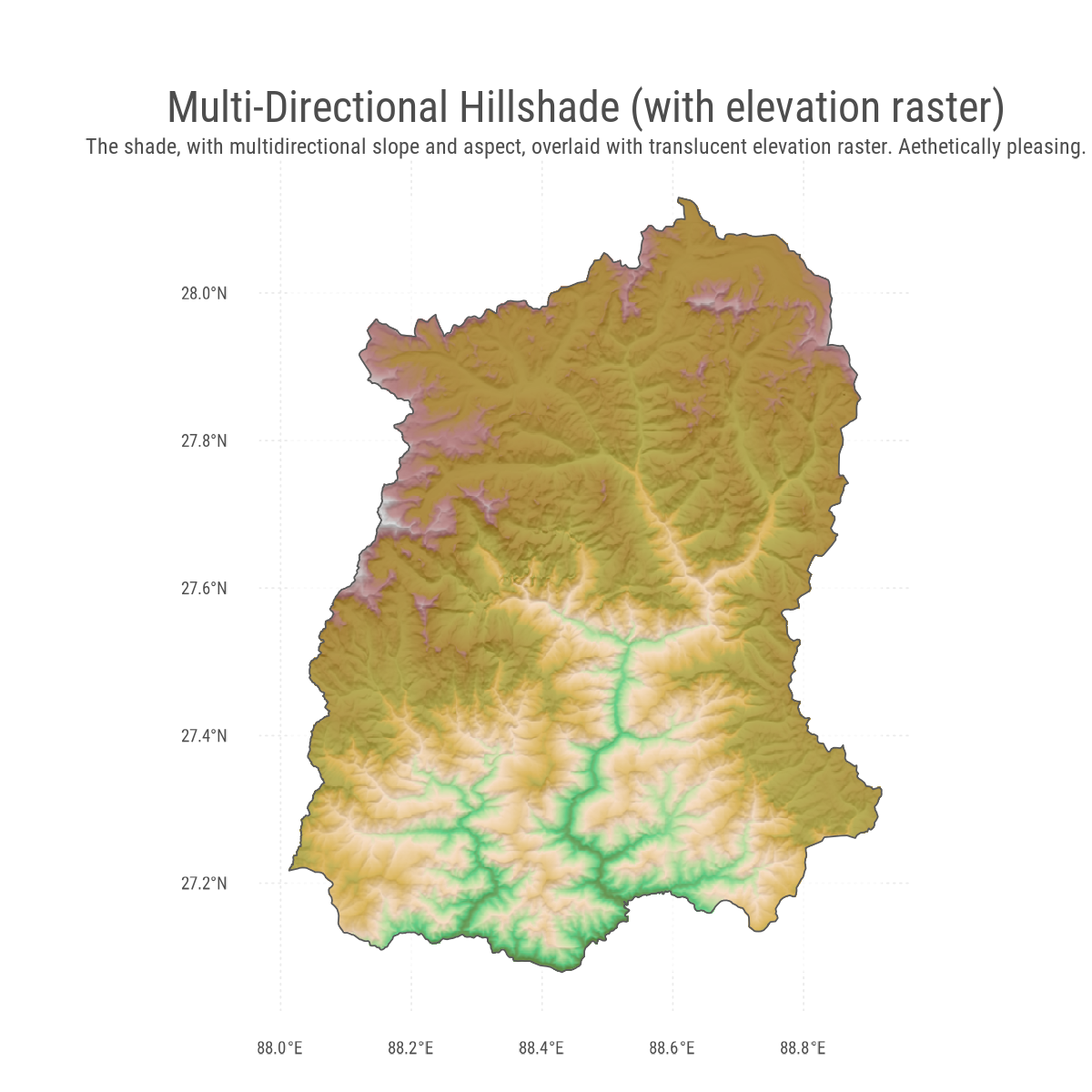
The following code generates a multi-directional hillshade effect for a raster dataset using the shade() function in the terra package. It applies shading from four different directions (270°, 15°, 60°, and 330°) to enhance topographic visualization. The outputs are combined into a single raster using rast() and summed up to create a composite hillshade. The ggplot2 package is then used to visualize the raster layers, with paletteer providing grayscale shading and ggnewscale enabling a second fill scale for an overlaid elevation raster. The sf package is used to add the outer boundary of Sikkim.

Code

# Multiple directions to shade() function
sikkim_shade_multi <- map(
  c(270, 15, 60, 330), 
  function(directions) {
    shade(
      slope1, 
      aspect1,
      angle = 45,
      direction = directions,
      normalize = TRUE
      )
    }
  )

# Create a multi-dimensional raster and reduce it by summing up
sikkim_shade_multi <- rast(sikkim_shade_multi) |> sum()

g4 <- ggplot() +
  
  geom_spatraster(
    data = sikkim_shade_multi
  ) +
  paletteer::scale_fill_paletteer_c(
    "grDevices::Light Grays",
    na.value = "transparent",
    direction = 1
  ) +
  # New fill scale
  ggnewscale::new_scale_fill() +
  
  # The elevation digital raster
  geom_spatraster(
    data = sikkim_rast,
    alpha = 0.7
  ) +
  scale_fill_hypso_c() +
  
  # Outer boundary map of Sikkim
  geom_sf(
    data = sikkim_vec,
    fill = NA
  ) +
  
  labs(
    title = "Multi-Directional Hillshade (with elevation raster)",
    subtitle = "The shade, with multidirectional slope and aspect, overlaid with translucent elevation raster. Aethetically pleasing."
  ) +
  theme(
    legend.position = "none",
    plot.title = element_text(
        size = bts * 2,
        margin = margin(15,0,2,0, "pt")
      ),
    plot.subtitle = element_text(
        size = bts,
        margin = margin(0,0,0,0, "pt")
      ),
    panel.grid = element_line(
        linewidth = 0.2,
        linetype = 3
    ),
    legend.title = element_text(
      margin = margin(0,0,2,0, "pt")
    ),
    legend.text = element_text(
      margin = margin(1,0,0,0, "pt")
    )
  )

ggsave(
  plot = g4,
  filename = here::here(
    "geocomputation", "images",
    "whitebox_terra_4.png"
  ),
  height = 1200,
  width = 1200,
  units = "px"
)

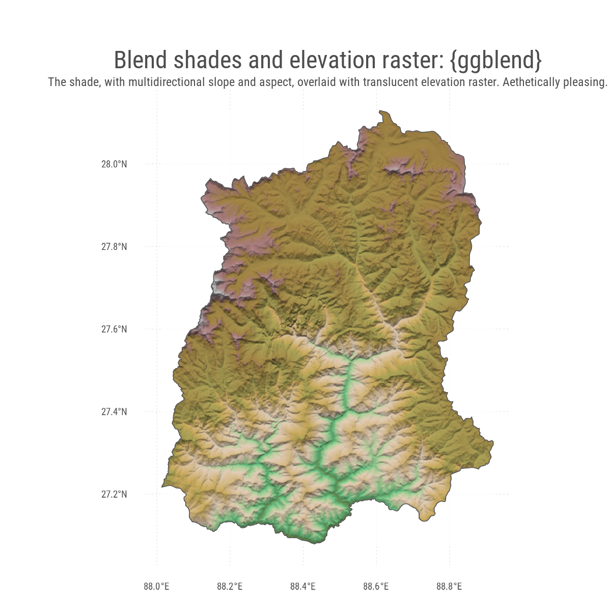
Blending Shades and Elevation Raster using `{ggblend}`

The following code creates a visually appealing map of Sikkim by blending a multidirectional hillshade raster with an elevation raster using {ggblend}. The geom_raster() function is used twice—first to plot the hillshade (sikkim_shade_multi) using a light gray palette from {paletteer}, and then to overlay a semi-transparent digital elevation model (sikkim_rast) with scale_fill_hypso_c(). The {ggnewscale} package allows a new fill scale for the second raster layer. The vector boundary of Sikkim is added using geom_sf(), and the final composition is styled using {ggplot2}’s theme().

Code

temp_tibble <- sikkim_rast |> as_tibble(xy = T)
names(temp_tibble) <- c("x", "y", "alt")

g5 <- ggplot() +

  (
    list(  
      # The shadows part of the raster map
      geom_raster(
        data = sikkim_shade_multi |> as.tibble(xy = T),
        aes(x, y, fill = sum)
      ),
      paletteer::scale_fill_paletteer_c(
        "grDevices::Light Grays",
        na.value = "transparent",
        direction = 1
      ),
      
      # New fill scale
      ggnewscale::new_scale_fill(),
      
      # The elevation digital raster
      geom_raster(
        data = temp_tibble,
        aes(x, y, fill = alt),
        alpha = 0.7
      ),
      scale_fill_hypso_c()
    ) |> blend("multiply")
  ) +
  
  # Outer boundary map of Sikkim
  geom_sf(
    data = sikkim_vec,
    fill = NA
  ) +
  coord_sf() +
  
  labs(
    title = "Blend shades and elevation raster: {ggblend}",
    subtitle = "The shade, with multidirectional slope and aspect, overlaid with translucent elevation raster. Aethetically pleasing.",
    x = NULL, y = NULL
  ) +
  theme(
    legend.position = "none",
    plot.title = element_text(
        size = bts * 2,
        margin = margin(15,0,2,0, "pt")
      ),
    plot.subtitle = element_text(
        size = bts,
        margin = margin(0,0,0,0, "pt")
      ),
    panel.grid = element_line(
        linewidth = 0.2,
        linetype = 3
    ),
    legend.title = element_text(
      margin = margin(0,0,2,0, "pt")
    ),
    legend.text = element_text(
      margin = margin(1,0,0,0, "pt")
    )
  )

ggsave(
  plot = g5,
  filename = here::here(
    "geocomputation", "images",
    "whitebox_terra_5.png"
  ),
  height = 1200,
  width = 1200,
  units = "px"
)

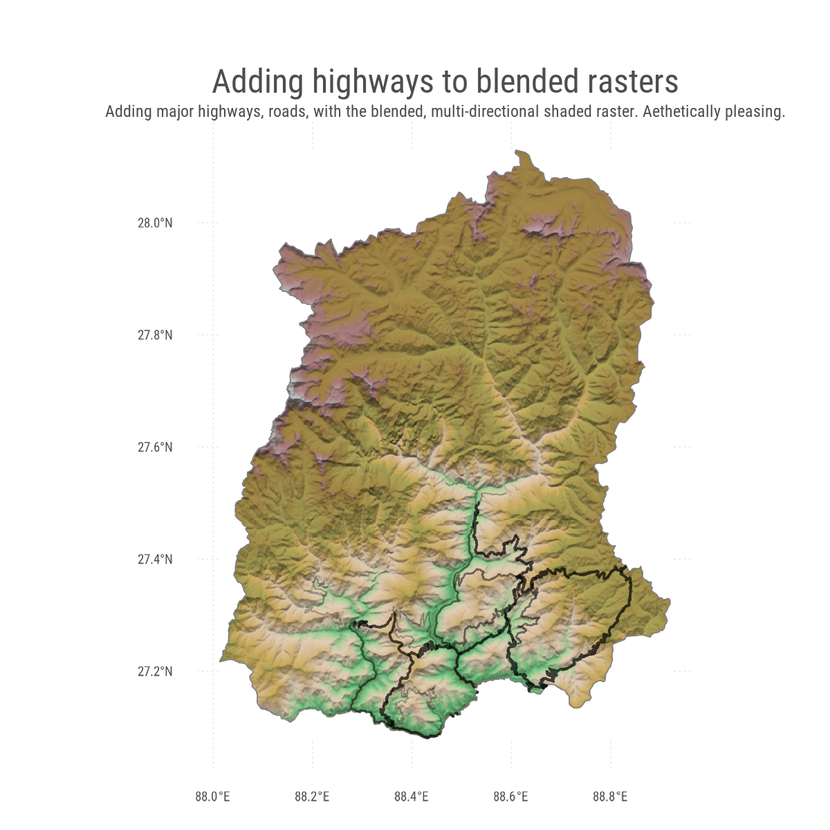
Creating a Blended Raster Map with Highways in Sikkim

The following code generates a visually appealing map of Sikkim by blending multiple raster layers and overlaying highway data. It uses ggplot2 for plotting, paletteer for color scales, and ggnewscale to introduce multiple fill scales. The base raster consists of a multi-directional shaded relief layer (sikkim_shade_multi) and an elevation raster (sikkim_rast), which are blended using the blend("multiply") function. The map also incorporates sf data layers for the Sikkim boundary (sikkim_vec) and major highways (sikkim_roads), with varying linewidths and alpha values set using scale_linewidth_manual() and scale_alpha_manual().

Code

g6 <- ggplot() +

  # A list for blended raster colours
  (
    list(  
      # The shadows part of the raster map
      geom_raster(
        data = sikkim_shade_multi |> as.tibble(xy = T),
        aes(x, y, fill = sum)
      ),
      paletteer::scale_fill_paletteer_c(
        "grDevices::Light Grays",
        na.value = "white",
        direction = 1
      ),
      
      # New fill scale
      ggnewscale::new_scale_fill(),
      
      # The elevation digital raster
      geom_raster(
        data = sikkim_rast |> as.tibble(xy = T),
        aes(x, y, fill = file32e432a33603),
        alpha = 0.7
      ),
      scale_fill_hypso_c()
    ) |> blend("multiply")
  ) +
  
  # Outer boundary map of Sikkim
  geom_sf(
    data = sikkim_vec,
    fill = NA,
    colour = "grey50"
  ) +
  coord_sf() +
  geom_sf(
    data = sikkim_roads,
    mapping = aes(
      linewidth = highway,
      alpha = highway
    )
  ) +
  scale_linewidth_manual(
    values = c(0.2, 0.3, 0.4)
  ) +
  scale_alpha_manual(
    values = c(0.3, 0.5, 0.7)
  ) +
  labs(
    title = "Adding highways to blended rasters",
    subtitle = "Adding major highways, roads, with the blended, multi-directional shaded raster. Aethetically pleasing.",
    x = NULL, y = NULL
  ) +
  theme(
    legend.position = "none",
    plot.title = element_text(
        size = bts * 2,
        margin = margin(15,0,2,0, "pt")
      ),
    plot.subtitle = element_text(
        size = bts,
        margin = margin(0,0,0,0, "pt")
      ),
    panel.grid = element_line(
        linewidth = 0.2,
        linetype = 3
    ),
    legend.title = element_text(
      margin = margin(0,0,2,0, "pt")
    ),
    legend.text = element_text(
      margin = margin(1,0,0,0, "pt")
    )
  )

ggsave(
  plot = g6,
  filename = here::here(
    "geocomputation", "images",
    "whitebox_terra_6.png"
  ),
  height = 1200,
  width = 1200,
  units = "px"
)

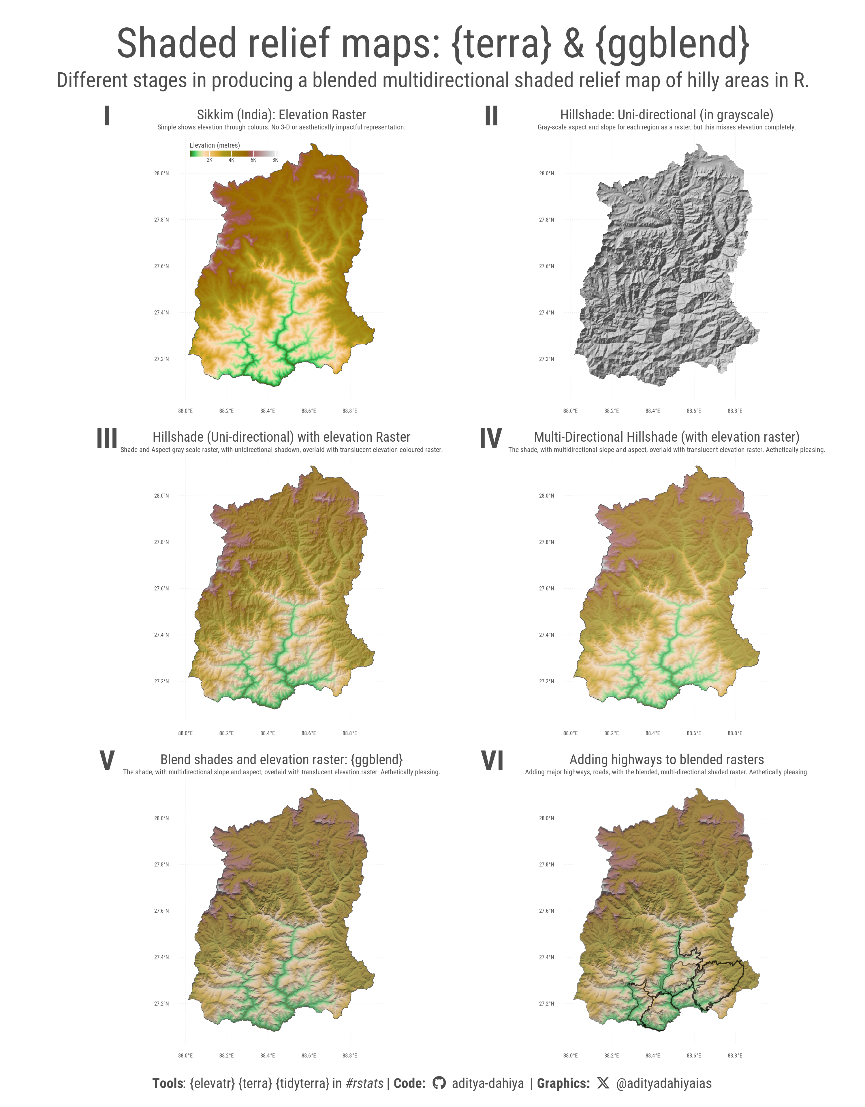
Creating a Multi-Panel Shaded Relief Map Layout

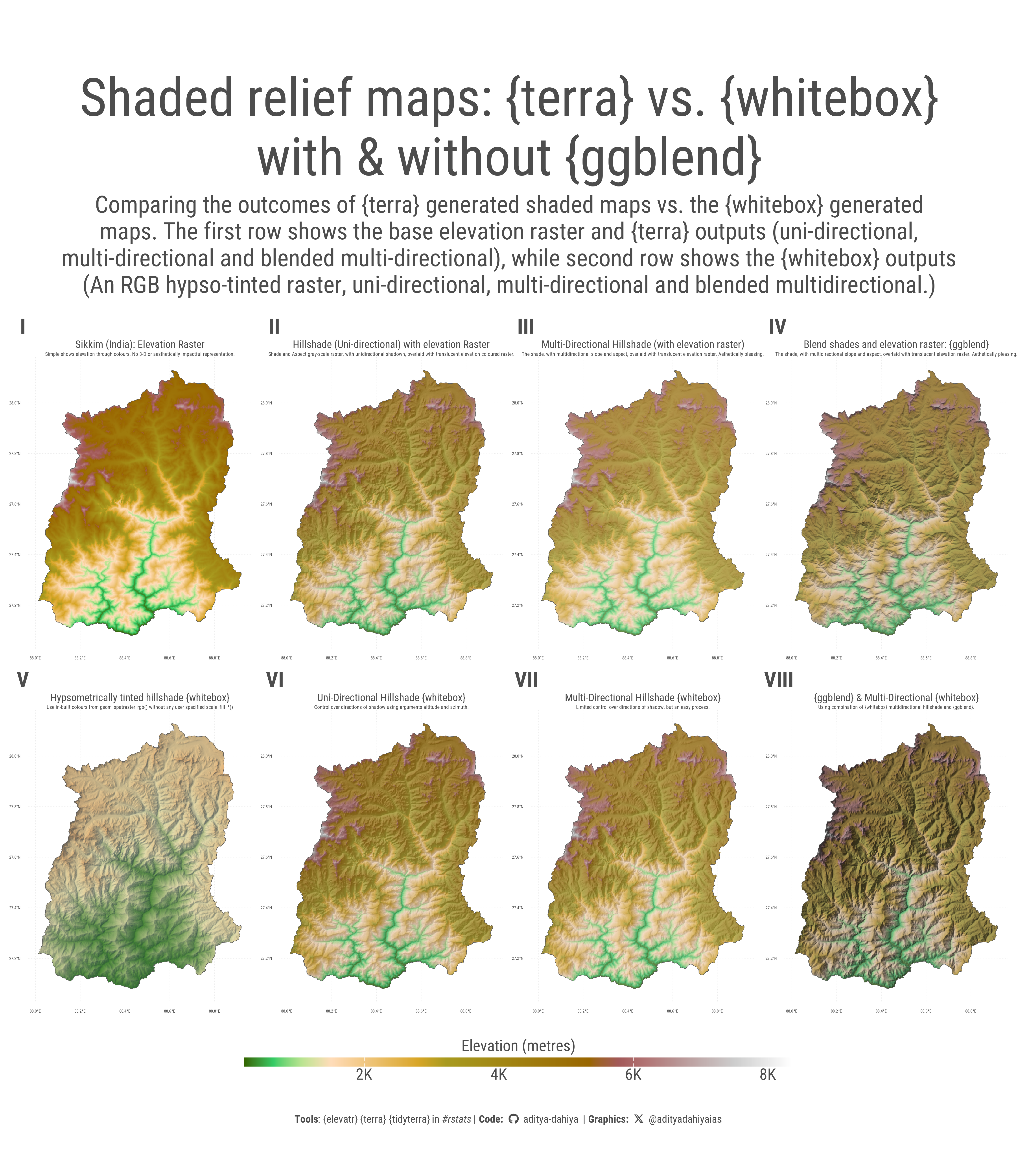
The following code uses the {patchwork} package to arrange multiple ggplot2 plots into a structured layout. It combines six plots (g1 to g6) using wrap_plots(), setting a 2-column by 3-row grid with plot_layout(). The {ggblend} and {terra} packages are referenced in the title to indicate the process of creating blended multidirectional shaded relief maps. The plot_annotation() function adds a title, subtitle, and caption, while theme() customizes text styles and margins.

Code

library(patchwork)

g <- wrap_plots(g1, g2, g3, g4, g5, g6) +
  plot_layout(
    ncol = 2,
    nrow = 3
  ) +
  plot_annotation(
    title = "Shaded relief maps: {terra} & {ggblend}",
    subtitle = "Different stages in producing a blended multidirectional shaded relief map of hilly areas in R.",
    caption = plot_caption,
    tag_levels = "I",
    theme = theme(
      plot.title = element_text(
        margin = margin(20,0,5,0, "pt"),
        size = bts * 6
      ),
      plot.subtitle = element_text(
        margin = margin(0,0,0,0, "pt"),
        size = bts * 3
      ),
      plot.caption = element_textbox(
        hjust = 0.5,
        size = bts * 2,
        margin = margin(15,0,10,0, "pt")
      )
    )
  ) &
  theme(
    plot.margin = margin(0,40,0,40, "pt"),
    plot.tag = element_text(
      size = bts * 4,
      face = "bold",
      margin = margin(0,30,-40,0, "pt")
    )
  )

ggsave(
  plot = g,
  filename = here::here(
    "geocomputation", "images",
    "whitebox_terra_7.png"
  ),
  height = 1200 * 3.2,
  width = 1200 * 2.5,
  units = "px",
  bg = "white"
)

Figure 7: A composite plot of the (I) the elevation raster of the height above sea level for the state of Sikkim (India). (II) A grey-scale hillshade graph showing the spect and slope, irrespective of the elevation. (III) The same map, but in a uni-directional shadow, now merged with translucent elevation raster. (IV) With a multi-drectional shade. (V) With a blended (using `ggblend`) colours from the grayscale shaded relief and coloured elevation raster. And, (VI) the blended raster with overlaid highways and roads.

An alternative for shaded relief maps: {whitebox}

This R script utilizes the {whitebox} package to generate a hillshade raster from a Digital Elevation Model (DEM) of Sikkim, India. Hillshade is a technique that simulates the illumination of a surface by a light source to accentuate terrain features, enhancing the visualization of topographic relief. The script begins by saving the DEM (sikkim_rast) as a TIFF file, as WhiteboxTools operates on TIFF inputs. It then initializes WhiteboxTools and applies the wbt_hillshade() function, specifying parameters such as azimuth (direction of the light source) and altitude (angle of the light source above the horizon) to control the illumination’s direction and angle. The resulting hillshade raster is subsequently masked using the vector boundaries of Sikkim (sikkim_vec) to limit the visualization to the area of interest. Finally, the script employs {ggplot2} to overlay the hillshade and elevation data, creating a composite map that effectively highlights the terrain’s features.

Code

# Install the package {whitebox}
# install.packages("whitebox")

# Load the library {whitebox}
library(whitebox)

# Download the 'WhiteboxTools' binary if needed.
# install_whitebox()


# Since Whitebox tools operate on .tiff files, save the raster
# as a tiff file first.

terra::writeRaster(
  x = sikkim_rast, 
  filename = here::here("geocomputation", "temp_sikkim.tiff"),
  overwrite = T
)

# Launch Whitebox
wbt_init()

whitebox::wbt_hillshade(
  dem = here::here("geocomputation", "temp_sikkim.tiff"),
  output = here::here("geocomputation", "temp_sikkim1.tiff"),
  azimuth = 315,
  altitude = 20
)

sikkim_wbt <- rast(
  here::here("geocomputation", "temp_sikkim1.tiff")
) |> 
  terra::mask(sikkim_vec)

g8 <- ggplot() +
  
  # WhiteBox Uni-directional Shadow
  geom_spatraster(data = sikkim_wbt) +
  paletteer::scale_fill_paletteer_c(
    "grDevices::Light Grays",
    na.value = "transparent",
    direction = 1
  ) +
  
  # New fill scale
  ggnewscale::new_scale_fill() +
  
  # The elevation digital raster
  geom_spatraster(
    data = sikkim_rast,
    alpha = 0.7
  ) +
  scale_fill_hypso_c() +
  
  # Outer boundary map of Sikkim
  geom_sf(
    data = sikkim_vec,
    fill = NA
  ) +
  
  labs(
    title = "Uni-Directional Hillshade {whitebox}",
    subtitle = "Control over directions of shadow using arguments altitude and azimuth."
  ) +
  theme(
    legend.position = "none",
    plot.title = element_text(
        size = bts * 2,
        margin = margin(15,0,2,0, "pt")
      ),
    plot.subtitle = element_text(
        size = bts,
        margin = margin(0,0,0,0, "pt")
      ),
    panel.grid = element_line(
        linewidth = 0.2,
        linetype = 3
    ),
    legend.title = element_text(
      margin = margin(0,0,2,0, "pt")
    ),
    legend.text = element_text(
      margin = margin(1,0,0,0, "pt")
    )
  )

ggsave(
  plot = g8,
  filename = here::here(
    "geocomputation", "images",
    "whitebox_terra_8.png"
  ),
  height = 1200,
  width = 1200,
  units = "px"
)

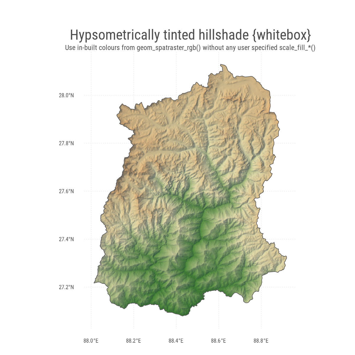
Hypsometrically tinted hill-shade

The provided R code utilizes the wbt_hypsometrically_tinted_hillshade function from the whitebox package to generate a hypsometrically tinted hillshade image of Sikkim, India. This function creates a color-shaded relief image from an input Digital Elevation Model (DEM) by combining hillshading with hypsometric tinting, which applies colors based on elevation ranges to enhance terrain visualization.

Code

whitebox::wbt_hypsometrically_tinted_hillshade(
  dem = here::here("geocomputation", "temp_sikkim.tiff"),
  output = here::here("geocomputation", "temp_sikkim1.tiff")
)

sikkim_wbt <- rast(
  here::here("geocomputation", "temp_sikkim1.tiff")
) |> 
  terra::mask(sikkim_vec)

g9 <- ggplot() +
  
  geom_spatraster_rgb(data = sikkim_wbt) +
  
  # Outer boundary map of Sikkim
  geom_sf(
    data = sikkim_vec,
    fill = NA
  ) +
  labs(
    title = "Hypsometrically tinted hillshade {whitebox}",
    subtitle = "Use in-built colours from geom_spatraster_rgb() without any user specified scale_fill_*()"
  ) +
  theme(
    legend.position = "none",
    plot.title = element_text(
        size = bts * 2,
        margin = margin(15,0,2,0, "pt")
      ),
    plot.subtitle = element_text(
        size = bts,
        margin = margin(0,0,0,0, "pt")
      ),
    panel.grid = element_line(
        linewidth = 0.2,
        linetype = 3
    ),
    legend.title = element_text(
      margin = margin(0,0,2,0, "pt")
    ),
    legend.text = element_text(
      margin = margin(1,0,0,0, "pt")
    )
  )

ggsave(
  plot = g9,
  filename = here::here(
    "geocomputation", "images",
    "whitebox_terra_9.png"
  ),
  height = 1200,
  width = 1200,
  units = "px"
)

Multidirectional hillshade

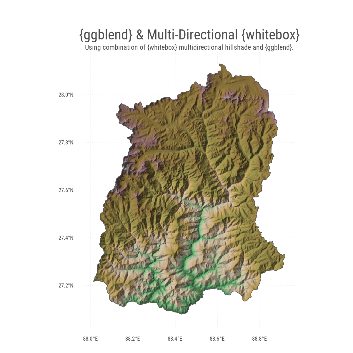
The provided R code utilizes the whitebox package to generate a multidirectional hillshade raster from a Digital Elevation Model (DEM) of Sikkim, India. The wbt_multidirectional_hillshade function calculates shading by considering illumination from multiple directions, resulting in a more detailed and realistic depiction of the terrain compared to traditional single-direction hillshade methods. In this code, the DEM is processed to produce a hillshade raster, which is then masked using the vector boundaries of Sikkim.

Code

whitebox::wbt_multidirectional_hillshade(
  dem = here::here("geocomputation", "temp_sikkim.tiff"),
  output = here::here("geocomputation", "temp_sikkim1.tiff"),
  altitude = 30
)

sikkim_wbt <- rast(
  here::here("geocomputation", "temp_sikkim1.tiff")
) |> 
  terra::mask(sikkim_vec)

ggsave(
  plot = g10,
  filename = here::here(
    "geocomputation", "images",
    "whitebox_terra_10.png"
  ),
  height = 1200,
  width = 1200,
  units = "px"
)

Blended Shades

Code

g12 <- ggplot() +
  
  # Start the blending
  (
    list(
      # WhiteBox Multidirectional Shadow
      geom_spatraster(data = sikkim_wbt),
      
      paletteer::scale_fill_paletteer_c(
        "grDevices::Light Grays",
        na.value = "transparent",
        direction = 1
      ),
      
      # New fill scale
      ggnewscale::new_scale_fill(),
      
      # The elevation digital raster
      geom_spatraster(
        data = sikkim_rast,
        alpha = 0.7
      ),
      scale_fill_hypso_c()
    ) |> blend("multiply")
  ) +
  
  # Outer boundary map of Sikkim
  geom_sf(
    data = sikkim_vec,
    fill = NA
  ) +
  
  labs(
    title = "{ggblend} & Multi-Directional {whitebox}",
    subtitle = "Using combination of {whitebox} multidirectional hillshade and {ggblend}."
  ) +
  theme(
    legend.position = "none",
    plot.title = element_text(
        size = bts * 2,
        margin = margin(15,0,2,0, "pt")
      ),
    plot.subtitle = element_text(
        size = bts,
        margin = margin(0,0,0,0, "pt")
      ),
    panel.grid = element_line(
        linewidth = 0.2,
        linetype = 3
    ),
    legend.title = element_text(
      margin = margin(0,0,2,0, "pt")
    ),
    legend.text = element_text(
      margin = margin(1,0,0,0, "pt")
    )
  )

ggsave(
  plot = g12,
  filename = here::here(
    "geocomputation", "images",
    "whitebox_terra_12.png"
  ),
  height = 1200,
  width = 1200,
  units = "px"
)

Compiling the Plots

Code

library(patchwork)

g1 <- g1 +
  theme(
    legend.position = "bottom",
      legend.direction = "horizontal",
      legend.key.height = unit(10, "pt"),
      legend.key.width = unit(120, "pt"),
      legend.title.position = "top",
      legend.text = element_text(
        size = 3 * bts,
        margin = margin(2,0,0,0, "pt")
        ),
      legend.title = element_text(
        size = 3 * bts,
        margin = margin(0,0,5,0, "pt"),
        hjust = 0.5
      )
  )
g11 <- wrap_plots(g1, g3, g4, g5, g9, g8, g10, g12) +
  plot_layout(
    ncol = 4,
    nrow = 2,
    guides = "collect"
  ) +
  plot_annotation(
    title = "Shaded relief maps: {terra} vs. {whitebox}\nwith & without {ggblend}",
    subtitle = str_wrap("Comparing the outcomes of {terra} generated shaded maps vs. the {whitebox} generated maps. The first row shows the base elevation raster and {terra} outputs (uni-directional, multi-directional and blended multi-directional), while second row shows the {whitebox} outputs (An RGB hypso-tinted raster, uni-directional, multi-directional and blended multidirectional.)", 95),
    caption = plot_caption,
    tag_levels = "I",
    theme = theme(
      plot.title = element_text(
        margin = margin(50,0,10,0, "pt"),
        size = bts * 10,
        lineheight = 0.3
      ),
      plot.subtitle = element_text(
        margin = margin(0,0,20,0, "pt"),
        size = bts * 4.5
      ),
      plot.caption = element_textbox(
        hjust = 0.5,
        size = bts * 2,
        margin = margin(15,0,10,0, "pt")
      ),
      legend.position = "bottom"
    )
  ) &
  theme(
    plot.margin = margin(0,5,10,5, "pt"),
    plot.tag = element_text(
      size = bts * 4,
      face = "bold",
      margin = margin(0,-30,-10,0, "pt")
    )
  )

ggsave(
  plot = g11,
  filename = here::here(
    "geocomputation", "images",
    "whitebox_terra_11.png"
  ),
  height = 1200 * 4.45,
  width = 1200 * 3.85,
  units = "px",
  bg = "white"
)

Final Compilation Plot - Comparing {terra} & {whitebox}

Figure 12: Final Compilation plot - comparing the two techniques

Trying the technique for Sikkim (India)

Elevation Raster Map

Grayscale Hillshade with Terrain Data

Uni-directional Shadow: with a Coloured raster map

Multi-Directional Hillshade with Elevation Raster

Blending Shades and Elevation Raster using {ggblend}

Creating a Blended Raster Map with Highways in Sikkim

Creating a Multi-Panel Shaded Relief Map Layout

An alternative for shaded relief maps: {whitebox}

Hypsometrically tinted hill-shade

Multidirectional hillshade

Blended Shades

Final Compilation Plot - Comparing {terra} & {whitebox}

Blending Shades and Elevation Raster using `{ggblend}`