Global Airports, Busiest Airports, Longest Flights
Maps
A4 Size Viz
Author
Aditya Dahiya
Published
May 19, 2024
Mapping the World’s Airports including the busiest; and the longest flights
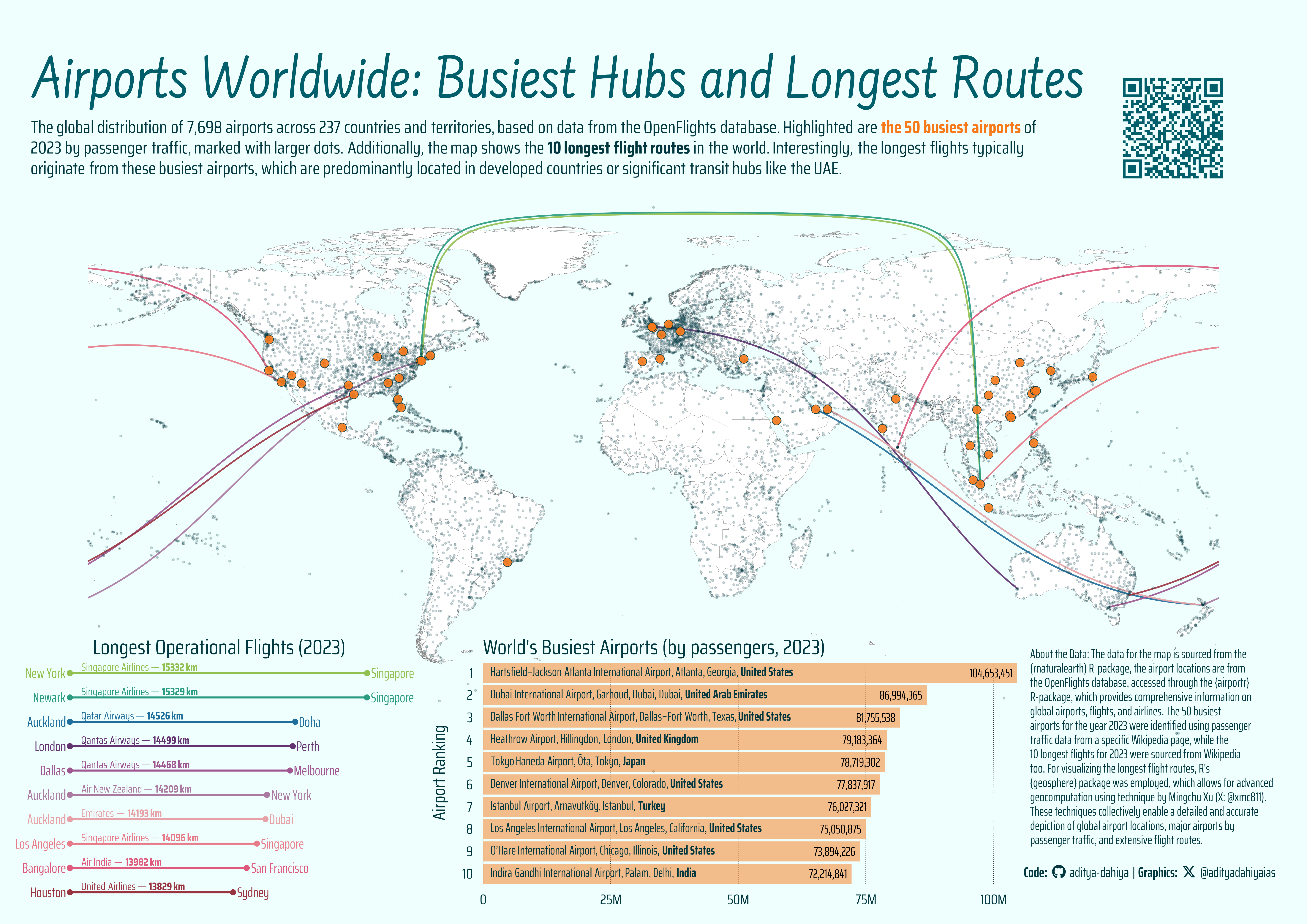
This comprehensive map provides a visual representation of the global aviation landscape, showcasing 7,698 airports across 237 countries and territories. The airport data is sourced from the OpenFlightsdatabase, accessible via the airportr package (Shkolnik 2019), which offers detailed information on over 15 million flights and more than 4,000 airlines. Additionally, the map highlights the 50 busiest airports of 2023, marked with larger orange dots, using passenger traffic data from Wikipedia. The 10 longest flight routes (data from OAG) are also depicted, plotted using R’s geosphere package (Hijmans 2022).
This visualization reveals that the longest flights often originate from the busiest airports, predominantly located in developed countries or major transit hubs like the UAE.
The global distribution of 7,698 airports across 237 countries and territories, based on data from the OpenFlights database. Highlighted are the 50 busiest airports of2023 by passenger traffic, marked with larger dots. Additionally, the map shows the 10 longest flight routes in the world. Interestingly, the longest flights typically originate from these busiest airports, which are predominantly located in developed countries or significant transit hubs like the UAE.
How I made this graphic?
Loading required libraries, data import & creating custom functions.
Code
# Data Import and Wrangling Toolslibrary(tidyverse) # All things tidy# Final plot toolslibrary(scales) # Nice Scales for ggplot2library(fontawesome) # Icons display in ggplot2library(ggtext) # Markdown text support for ggplot2library(showtext) # Display fonts in ggplot2library(colorspace) # Lighten and Darken colourslibrary(ggthemes) # Themes for ggplot2library(patchwork) # Combining plots# Mapping toolslibrary(sf) # All spatial objects in Rlibrary(airportr) # Airports Data for the worldlibrary(rnaturalearth) # World Map# Data on Airports: R Package airportr# https://cran.r-project.org/web/packages/airportr/vignettes/Introduction_to_Airportr.html
Data Analysis, Wrangling and web-scraping for additional datapoints
Code
# Names of airports around the worlddf <- airportr::airports |> janitor::clean_names() |>select(name, iata, city, country, cc2 = country_code_alpha_2, latitude,lat = latitude, lon = longitude) |>rename(airport = name) |>mutate(latitude = lat, longitude = lon) |>st_as_sf(coords =c("lon", "lat"), crs =4326)# List of 10 longest flights in the worldlongest_flights <-tibble(from =c("JFK", "EWR", "AKL", "LHR", "DFW","AKL", "AKL", "LAX", "BLR", "IAH"),to =c("SIN", "SIN", "DOH", "PER", "MEL","JFK", "DXB", "SIN", "SFO", "SYD"),airlines =c("Singapore Airlines", "Singapore Airlines","Qatar Airways", "Qantas Airways","Qantas Airways", "Air New Zealand","Emirates", "Singapore Airlines", "Air India", "United Airlines"),distance =c(15332, 15329, 14526, 14499, 14468,14209, 14193, 14096, 13982, 13829))# Extracting the busiest airports in the worldlibrary(rvest)# Define the URL of the Wikipedia pageurl <-"https://en.wikipedia.org/wiki/List_of_busiest_airports_by_passenger_traffic"# Read the HTML content of the page and# Extract the table with the 2023 statisticsbusiest_airports <-read_html(url) |>html_node(xpath ='//*[@id="mw-content-text"]/div[1]/table[1]') %>%html_table(fill =TRUE) |>as_tibble() |> janitor::clean_names() |>separate_wider_delim(cols = code_iata_icao,delim ="/",names =c("iata", "icao") ) |>select(-rankchange, -percent_change) |>mutate(totalpassengers =parse_number(totalpassengers))# Plotting the longest routes in the worldlongest_routes <- longest_flights |>left_join(df |>select(from = iata, from_lat = latitude, from_lon = longitude) |>as_tibble() |>select(-geometry)) |>left_join(df |>select(to = iata, to_lat = latitude, to_lon = longitude) |>as_tibble() |>select(-geometry))longest_route_airports <-unique(longest_routes$from, longest_routes$to)# Technique Credits: https://github.com/xmc811/flightplot/blob/master/R/main.R# Credits: Mingchu Xu# https://www.linkedin.com/in/mingchu-xu-467a0946/# On Twitter: @xmc811routes <- geosphere::gcIntermediate(p1 = longest_routes |>select(from_lon, from_lat),p2 = longest_routes |>select(to_lon, to_lat),n =1000,breakAtDateLine =TRUE,addStartEnd =TRUE,sp =TRUE) |> sf::st_as_sf() |>mutate(rank =row_number())# Test Plot# ggplot() +# geom_sf(# data = ne_countries(returnclass = "sf") |> # filter(sovereignt != "Antarctica"),# fill = "white"# ) +# geom_sf(# data = routes# ) +# coord_sf(crs = "ESRI:54030") +# ggthemes::theme_map()# Joining Airports Dataset with the busiest airports datasetplotdf <- df |>left_join(busiest_airports) |>mutate(busiest = iata %in% busiest_airports$iata,longest = iata %in% longest_route_airports,alpha_var = iata %in%c(busiest_airports$iata, longest_route_airports) ) |>mutate(totalpassengers =replace_na(totalpassengers, 1e7)) |>arrange(alpha_var)
Visualization Parameters
Code
# Font for titlesfont_add_google("Farsan",family ="title_font") # Font for the captionfont_add_google("Saira Extra Condensed",family ="caption_font") # Font for plot textfont_add_google("Saira Condensed",family ="body_font") showtext_auto()# Background Colourmypal <-c("#188a8d", "#ebfcfa", "white", "#013840", "#f77919")# orange_palette <- paletteer::paletteer_c(# "grDevices::Oranges", # n = 30)[8:17]orange_palette <- paletteer::paletteer_d("MetBrewer::Signac", direction =-1)[1:10]bg_col <- mypal[2] |>lighten(0.5)# Colour for the text using FAA's offical website colourtext_col <- mypal[4] # Colour for highlighted texttext_hil <-"#005f6b"text_hil2 <- mypal[5]# Define Base Text Sizets <-70# Caption stuff for the plotsysfonts::font_add(family ="Font Awesome 6 Brands",regular = here::here("docs", "Font Awesome 6 Brands-Regular-400.otf"))github <-""github_username <-"aditya-dahiya"xtwitter <-""xtwitter_username <-"@adityadahiyaias"social_caption_1 <- glue::glue("<span style='font-family:\"Font Awesome 6 Brands\";'>{github};</span> <span style='color: {text_col}'>{github_username} </span>")social_caption_2 <- glue::glue("<span style='font-family:\"Font Awesome 6 Brands\";'>{xtwitter};</span> <span style='color: {text_col}'>{xtwitter_username}</span>")
Plot Text
Code
plot_title <-"Airports Worldwide: Busiest Hubs and Longest Routes"plot_caption <-paste0("**Code:** ", social_caption_1, " | **Graphics:** ", social_caption_2 )plot_subtitle <- glue::glue("The global distribution of 7,698 airports across 237 countries and territories, based on data from the OpenFlights database. Highlighted are <b style='color:{mypal[5]}'>the 50 busiest airports</b> of<br>2023 by passenger traffic, marked with larger dots. Additionally, the map shows the <b>10 longest flight routes</b> in the world. Interestingly, the longest flights typically<br>originate from these busiest airports, which are predominantly located in developed countries or significant transit hubs like the UAE.")text_annotation_1 <-"About the Data: The data for the map is sourced from the {rnaturalearth} R-package, the airport locations are from the OpenFlights database, accessed through the {airportr} R-package, which provides comprehensive information on global airports, flights, and airlines. The 50 busiest airports for the year 2023 were identified using passenger traffic data from a specific Wikipedia page, while the 10 longest flights for 2023 were sourced from Wikipedia too. For visualizing the longest flight routes, R's {geosphere} package was employed, which allows for advanced geocomputation using technique by Mingchu Xu (X: @xmc811). These techniques collectively enable a detailed and accurate depiction of global airport locations, major airports by passenger traffic, and extensive flight routes."
Base Plot
Code
# Final Plot: A Composite world map with all Airports and # the busiest Airports in big size (with name and annual passengers)# And, in a different colour, the 10 longest flightsg_base <-ggplot() +geom_sf(data = world_map,fill = mypal[3],colour ="grey50",linewidth =0.1 ) +geom_sf(data = india_map,fill = mypal[3],colour ="grey50",linewidth =0.2 ) +geom_sf(data = routes,mapping =aes(colour =as_factor(rank)),alpha =0.9,linewidth =1 ) +scale_colour_manual(values = orange_palette) + ggnewscale::new_scale_colour() +geom_sf(data = plotdf,mapping =aes(fill = busiest,size = busiest,alpha = alpha_var ),colour = mypal[4],pch =21 ) +scale_fill_manual(values =c(mypal[4], mypal[5])) +scale_alpha_manual(values =c(0.2, 0.9)) +scale_size_manual(values =c(1, 5)) +# coord_sf(crs = "ESRI:54030") +coord_sf(ylim =c(-90, 90)) +labs(title = plot_title,subtitle = plot_subtitle,caption = plot_caption ) + ggthemes::theme_map(base_family ="body_font",base_size = ts ) +theme(plot.background =element_rect(fill = bg_col,colour ="transparent" ),panel.background =element_rect(fill = bg_col,colour ="transparent" ),legend.position ="none",plot.title =element_text(family ="title_font",hjust =0,colour = text_hil,size =3.6* ts,margin =margin(5,0,5,0, "mm") ),plot.subtitle =element_markdown(family ="body_font",lineheight =0.38,hjust =0,colour = text_col,margin =margin(0,0,0,0, "mm") ),plot.caption =element_textbox(hjust =1,family ="caption_font",colour = text_col,margin =margin(30,0,0,0, "mm") ) )
g <- g_base +# Add inset1 to the plotinset_element(p = inset1, left =0.33, right =0.78,bottom =0,top =0.3, align_to ="full",clip =FALSE,on_top =TRUE ) +# Add inset2 to the plotinset_element(p = inset2, left =0, right =0.33,bottom =0,top =0.3, align_to ="full",clip =FALSE,on_top =TRUE ) +# Add text inset to the plotinset_element(p = text_inset, left =0.58, right =1,bottom =0.08,top =0.28, align_to ="full",clip =TRUE,on_top =TRUE ) +# Add QR Code to the plotinset_element(p = plot_qr, left =0.85, right =0.95,bottom =0.8,top =0.95, align_to ="full",clip =FALSE ) +# Basix Plot Annotationsplot_annotation(theme =theme(plot.background =element_rect(fill = bg_col, colour =NA, linewidth =0 ) ) )