All the places - brands & stores around the world

Template for future Visualizations

All the places

All the Places is a project aimed at generating point of interest (POI) data by sourcing information from websites with ‘store location’ pages. The project utilizes scrapy, a popular Python-based web scraping framework, to run individual site spiders that extract POI data. The results are then published in a standard format. There are several scrapy tutorials available on-line, and this series on YouTube provides a reasonable starting point.

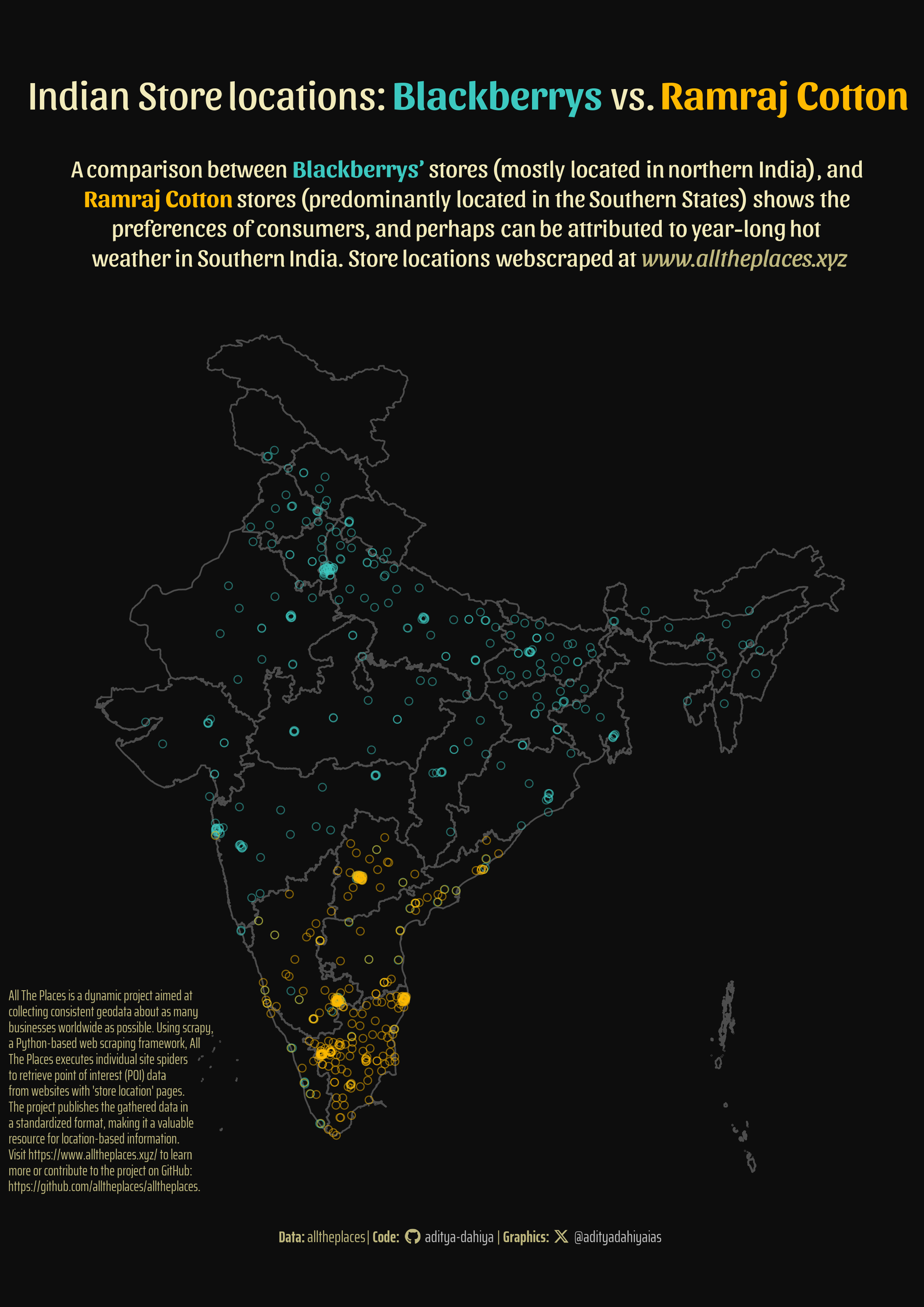
Comparing Store Locations for Blackberrys and Ramraj Cotton in India

How I made this graphic?

Loading required libraries, data import & creating custom functions

# Data Import and Wrangling Tools
library(tidyverse)            # All things tidy
library(janitor)              # Cleaning names etc.

# Final plot tools
library(scales)               # Nice Scales for ggplot2
library(fontawesome)          # Icons display in ggplot2
library(ggtext)               # Markdown text support for ggplot2
library(showtext)             # Display fonts in ggplot2
library(colorspace)           # Lighten and Darken colours
library(ggthemes)             # Themes for ggplot2
library(patchwork)            # Combining plots
library(ggfx)                 # Outer glow in the map
library(magick)               # Adding images to plot

# Mapping tools
library(rnaturalearth)        # Maps of the World   
library(sf)                   # All spatial objects in R
library(geojsonio)            # To read geojson files into R


# Importing raw data: Ramraj Cotton
name_of_store1 <- "ramraj_cotton_in"
url1 <- paste0(
  "https://alltheplaces-data.openaddresses.io/runs/2024-04-20-13-31-46/output/", 
  name_of_store1, 
  ".geojson")

df1 <- geojsonio::geojson_read(url1, what = "sp") |> 
  st_as_sf(crs = 4326) |> 
  janitor::clean_names() |> 
  mutate(store_name = "Ramraj Cotton")

# Importing raw data: Blackberrys India
name_of_store2 <- "blackberrys_in"
url2 <- paste0(
  "https://alltheplaces-data.openaddresses.io/runs/2024-04-20-13-31-46/output/", 
  name_of_store2, 
  ".geojson")

df2 <- geojsonio::geojson_read(url2, what = "sp") |> 
  st_as_sf(crs = 4326) |> 
  janitor::clean_names() |> 
  mutate(store_name = "Blackberrys")

rm(url1, url2, name_of_store)

# Map of India with states
india_map <- read_sf(here::here("data", "india_map", "India_State_Boundary.shp")) |> 
  st_simplify(dTolerance = 100)

# An outer map of India to have a glow
india_outer_map <- read_sf(here::here("data", "india_map", "India_State_Boundary.shp")) |> 
  st_simplify(dTolerance = 100) |> 
  rmapshaper::ms_dissolve() |>             # removing the internal state borders
  rmapshaper::ms_simplify(keep = 0.05)     # removing left over multiploygons

Visualization Parameters

# Font for titles
font_add_google("Sansita",
  family = "title_font"
) 

# Font for the caption
font_add_google("Saira Extra Condensed",
  family = "caption_font"
) 

# Font for plot text
font_add_google("Amita",
  family = "body_font"
) 

showtext_auto()

# Background Colour
bg_col <- "grey5"

# Colour for the text
text_col <- "#F2EBBBFF" 

# Colour for highlighted text
text_hil <- "#F2EBBBFF" 

# Colour for brands
col_bb <- "#FFA400FF"
col_rc <- "#862633FF"

# Define Base Text Size
ts <- 40 

# Caption stuff for the plot
sysfonts::font_add(
  family = "Font Awesome 6 Brands",
  regular = here::here("docs", "Font Awesome 6 Brands-Regular-400.otf")
)
github <- "&#xf09b"
github_username <- "aditya-dahiya"
xtwitter <- "&#xe61b"
xtwitter_username <- "@adityadahiyaias"
social_caption_1 <- glue::glue("<span style='font-family:\"Font Awesome 6 Brands\";'>{github};</span> <span style='color: {text_hil}'>{github_username}  </span>")
social_caption_2 <- glue::glue("<span style='font-family:\"Font Awesome 6 Brands\";'>{xtwitter};</span> <span style='color: {text_hil}'>{xtwitter_username}</span>")

Annotation Text for the Plot

plot_title <- glue::glue("Indian Store locations: <b style='color:{col_bb}'>Blackberrys</b> vs. <b style='color:{col_rc}'>Ramraj Cotton</b>")

plot_caption <- paste0(
  "**Data:** alltheplaces", 
  " |  **Code:** ", 
  social_caption_1, 
  " |  **Graphics:** ", 
  social_caption_2
  )

plot_subtitle <- glue::glue("A comparison between <b style='color:{col_bb}'>Blackberrys'</b> stores (mostly located in northern India), and <br><b style='color:{col_rc}'>Ramraj Cotton</b> stores (predominantly located in the Southern States) shows the <br>preferences of consumers, and perhaps can be attributed to year-long hot <br>weather in Southern India. Store locations webscraped at <i style='color:{text_hil}'>www.alltheplaces.xyz</i>")

Plot on the map of India

# Background Colour
bg_col <- "grey5"

# Colour for the text
text_col <- "#F2EBBBFF" 

# Colour for highlighted text
text_hil <- "#F2EBBBFF" |> darken(0.2)

# Colour for brands
col_bb <- "#3CC8C0FF"
col_rc <- "#FFB900FF"

g_base <- ggplot(
  data = df1,
  mapping = aes(colour = store_name)
) +
  # with_outer_glow(
  #   geom_sf(
  #     data = india_outer_map,
  #     colour = "grey30",
  #     linewidth = 0.5,
  #     fill = "transparent"
  #   ),
  #   colour = "grey30",
  #   sigma = 30
  # ) +
  geom_sf(
      data = india_map,
      colour = "grey30",
      linewidth = 0.5,
      fill = "transparent"
    ) +
  geom_sf(
    data = df2,
    alpha = 0.5,
    pch = 1, 
    fill = "transparent",
    size = 2
  ) +
  geom_sf(
    data = df1,
    alpha = 0.5,
    pch = 1, 
    fill = "transparent",
    size = 2
  ) +
  scale_colour_manual(values = c(col_bb, col_rc)) +
  labs(
    title = plot_title,
    subtitle = plot_subtitle,
    caption = plot_caption
  ) +
  theme_map(base_size = 40) +
  theme(
    plot.background = element_rect(
      fill = bg_col,
      linewidth = NA, 
      colour = NA
    ),
    plot.title = ggtext::element_markdown(
      size = 2 * ts,
      colour = text_col,
      family = "title_font",
      margin = margin(10, 0, 5, 0,"mm"),
      hjust = 0.5,
      lineheight = 0.35
    ),
    plot.subtitle = ggtext::element_markdown(
      hjust = 0.5, 
      lineheight = 0.4,
      colour = text_col,
      family = "title_font",
      margin = margin(5, 0, 5, 0, "mm"),
      size = 1.2 * ts
    ),
    plot.caption = ggtext::element_textbox(
      hjust = 0.5,
      family = "caption_font",
      colour = text_hil,
      margin = margin(0, 0, 5, 0, "mm")
    ),
    legend.position = "none"
  )

Add-on maps, insets and annotations

inset1 <- ggplot() +
  annotate(
    geom = "text",
    x = 0,
    y = 0,
    label = str_wrap("All The Places is a dynamic project aimed at collecting consistent geodata about as many businesses worldwide as possible. Using scrapy, a Python-based web scraping framework, All The Places executes individual site spiders to retrieve point of interest (POI) data from websites with 'store location' pages. The project publishes the gathered data in a standardized format, making it a valuable resource for location-based information. Visit https://www.alltheplaces.xyz/ to learn more or contribute to the project on GitHub: https://github.com/alltheplaces/alltheplaces.", 50),
    colour = text_hil,
    family = "caption_font",
    size = 10,
    lineheight = 0.3,
    hjust = 0,
    vjust = 1
  ) +
  theme_void()

# image_bb_url <- "https://blackberrys.com/cdn/shop/files/LOGOheaderenew.png"
# 
# image_read(image_bb_url) |> 
#   image_
#   image_background(color = bg_col)

Compiling Plots with Patchwork

g <- g_base + 
  
  # Add inset to the plot
  inset_element(
    p = inset1, 
    left = -0.3, 
    right = 0.22,
    bottom = 0.01,
    top = 0.5, 
    align_to = "plot"
  ) +
  
  # Basix Plot Annotations
  plot_annotation(
    theme = theme(
      plot.background = element_rect(
        fill = bg_col, 
        colour = NA, linewidth = 0
      )
    )
  )

Savings the graphics

ggsave(
  filename = here::here("data_vizs", "all_the_places.png"),
  plot = g,
  width = 210,    # Default A4 size page
  height = 297,   # Default A4 size page
  units = "mm",
  bg = bg_col
)


library(magick)
# Saving a thumbnail for the webpage
image_read(here::here("data_vizs", "all_the_places.png")) |> 
  image_resize(geometry = "400") |> 
  image_write(here::here("data_vizs", "thumbnails", "all_the_places.png"))

Future Work Plan: Glowing colours; Add Glow to outer borders