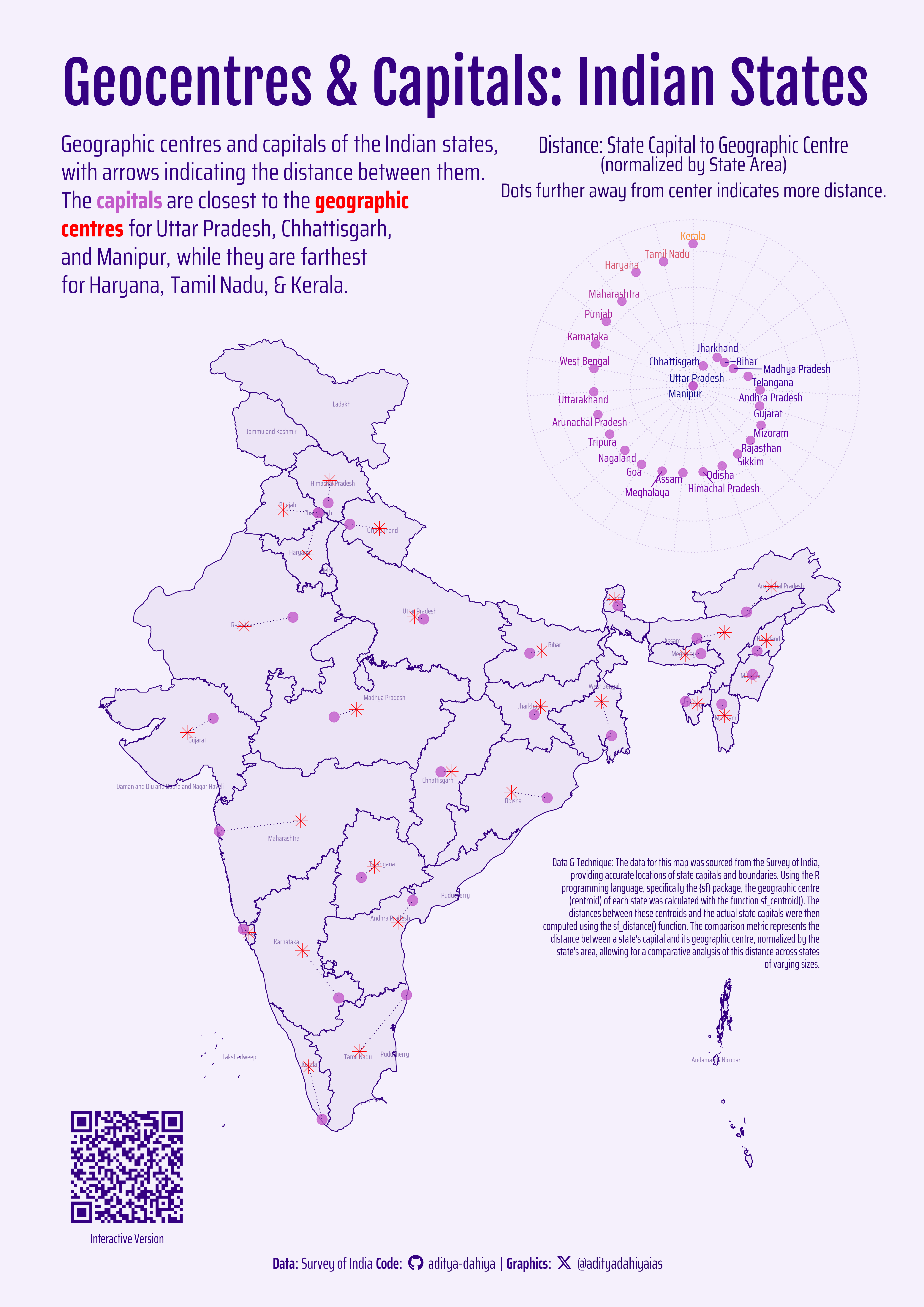
How Far Are Indian Capitals from Their Geographic Centres?
This map analyzes the spatial relationship between state capitals and their geographic centres in India, revealing which capitals are closest and farthest from their central points when adjusted for state area.
A4 Size Viz
India
Maps
Interactive
The map illustrates the geographic centres and capitals of Indian states, based on data from the Survey of India. Using the R programming language and the sf package (Pebesma and Bivand 2023) , the geographic centres were determined with the sf_centroid() function, and distances to the capitals were calculated using sf_distance(). These distances were normalized by the square root of the state area to allow for meaningful comparisons across states of varying sizes. The findings show that the capitals of Uttar Pradesh, Chhattisgarh, and Manipur are closest to their geographic centres, while those of Haryana, Tamil Nadu, and Kerala are the farthest. This spatial relationship is visually represented with arrows connecting the geographic centres to the state capitals.
Interactive Version of the map
How I made this graphic?
Getting the data
Code
# Data Import and Wrangling Tools
library(tidyverse)            # All things tidy

# Final plot tools
library(scales)               # Nice Scales for ggplot2
library(fontawesome)          # Icons display in ggplot2
library(ggtext)               # Markdown text support for ggplot2
library(showtext)             # Display fonts in ggplot2
library(colorspace)         # To lighten and darken colours

# Maps related packages
library(sf)                   # Geomteric objects manipulation

# Get State Map of India
india_state_map <- read_sf(here::here(
  "data", "india_map", "India_State_Boundary.shp"
)) |>
  # During interations, using lower resolution for quick plotting
  # st_simplify(dTolerance = 5000) |>
  st_transform(crs = 4326) |>
  mutate(state = case_when(
    State_Name == "Chhattishgarh" ~ "Chhattisgarh",
    State_Name == "Tamilnadu" ~ "Tamil Nadu",
    State_Name == "Telengana" ~ "Telangana",
    .default = State_Name
    ),
    .keep = "unused"
  )

state_capitals <- tibble(
  State = c(
    "Andhra Pradesh", "Arunachal Pradesh", "Assam", "Bihar",
    "Chhattishgarh", "Goa", "Gujarat", "Haryana", "Himachal Pradesh",
    "Jharkhand", "Karnataka", "Kerala", "Madhya Pradesh",
    "Maharashtra", "Manipur", "Meghalaya", "Mizoram", "Nagaland",
    "Odisha", "Punjab", "Rajasthan", "Sikkim", "Tamilnadu",
    "Telengana", "Tripura", "Uttar Pradesh", "Uttarakhand",
    "West Bengal"),
  Capital = c(
    "Amaravati", "Itanagar", "Dispur", "Patna", "Raipur",
    "Panaji", "Gandhinagar", "Chandigarh", "Shimla", "Ranchi",
    "Bengaluru", "Thiruvananthapuram", "Bhopal", "Mumbai", "Imphal",
    "Shillong", "Aizawl", "Kohima", "Bhubaneswar", "Chandigarh",
    "Jaipur", "Gangtok", "Chennai", "Hyderabad", "Agartala",
    "Lucknow", "Dehradun", "Kolkata"),
  Latitude = c(16.5417, 27.1020, 26.1445, 25.5941, 21.2514,
               15.4909, 23.2156, 30.7333, 31.1048, 23.3441,
               12.9716, 8.5241, 23.2599, 19.0760, 24.8170,
               25.5788, 23.7271, 25.6751, 20.2961, 30.7333,
               26.9124, 27.3314, 13.0827, 17.3850, 23.8315,
               26.8467, 30.3165, 22.5726),
  Longitude = c(80.5167, 93.6920, 91.7362, 85.1376, 81.6296,
                73.8278, 72.6369, 76.7794, 77.1734, 85.3096,
                77.5946, 76.9366, 77.4126, 72.8777, 93.9368,
                91.8933, 92.7176, 94.1086, 85.8245, 76.7794,
                75.7873, 88.6138, 80.2707, 78.4867, 91.2868,
                80.9462, 78.0322, 88.3639)
)
Visualization Parameters
Code
# Font for titles
font_add_google("Fjalla One",
family = "title_font"
)
# Font for the caption
font_add_google("Saira Extra Condensed",
family = "caption_font"
)
# Font for plot text
font_add_google("Saira Condensed",
family = "body_font"
)
showtext_auto()
# Background Colour
bg_col <- "#f5f0fc"
text_col <- "#2a0169"
text_hil <- "#350182"
viz_cols <- paletteer::paletteer_d("ltc::trio1")
viz_cols[2] <- "red"
# Base Text Size
bts <- 80
plot_title <- "Geocentres & Capitals: Indian States"
plot_subtitle <- glue::glue("Geographic centres and capitals of the Indian states,<br>with arrows indicating the distance between them.<br>The <b style='color:{viz_cols[3] }'>capitals</b> are closest to the <b style='color:{viz_cols[2] }'>geographic</b><br><b style='color:{viz_cols[2] }'>centres</b> for Uttar Pradesh, Chhattisgarh,<br>and Manipur, while they are farthest<br>for Haryana, Tamil Nadu, & Kerala.")
# Caption stuff for the plot
sysfonts::font_add(
family = "Font Awesome 6 Brands",
regular = here::here("docs", "Font Awesome 6 Brands-Regular-400.otf")
)
social_caption_1 <- glue::glue("<span style='font-family:\"Font Awesome 6 Brands\";'></span> <span style='color: {text_col}'>aditya-dahiya </span>")
social_caption_2 <- glue::glue("<span style='font-family:\"Font Awesome 6 Brands\";'></span> <span style='color: {text_col}'>@adityadahiyaias </span>")
plot_caption <- paste0(
"**Data:** Survey of India ",
"**Code:** ", social_caption_1,
" | **Graphics:** ", social_caption_2
)
data_source <- str_wrap("Data & Technique: The data for this map was sourced from the Survey of India, providing accurate locations of state capitals and boundaries. Using the R programming language, specifically the {sf} package, the geographic centre (centroid) of each state was calculated with the function sf_centroid(). The distances between these centroids and the actual state capitals were then computed using the sf_distance() function. The comparison metric represents the distance between a state's capital and its geographic centre, normalized by the state's area, allowing for a comparative analysis of this distance across states of varying sizes.", 80)
data_source |> str_view()Data Wrangling
Code
# Calculate geomteric centres of each state
df1 <- india_state_map |>
  st_centroid() |>
  rename(geometry_centroid = geometry)

df1 <- df1 |>
  mutate(
    from_lon = sf::st_coordinates(df1)[,1],
    from_lat = sf::st_coordinates(df1)[,2]) |>
    as_tibble() |>
    mutate(state = case_when(
    state == "Chhattishgarh" ~ "Chhattisgarh",
    state == "Tamilnadu" ~ "Tamil Nadu",
    state == "Telengana" ~ "Telangana",
    .default = state
    ),
    .keep = "unused"
  )
print(df1, n = Inf)

# Capitals of each state
df2 <- state_capitals |>
  janitor::clean_names() |>
  st_as_sf(coords = c("longitude", "latitude")) |>
  rename(
    State_Name = state,
    geometry_capital = geometry
  )

df2 <- df2 |>
  mutate(
    to_lon = sf::st_coordinates(df2)[,1],
    to_lat = sf::st_coordinates(df2)[,2]
  ) |>
  as_tibble() |>
  rename(state = State_Name) |>
  mutate(state = case_when(
    state == "Chhattishgarh" ~ "Chhattisgarh",
    state == "Tamilnadu" ~ "Tamil Nadu",
    state == "Telengana" ~ "Telangana",
    .default = state
    ),
    .keep = "unused"
  )

print(df2, n = Inf)

plotdf <- df2 |>
  left_join(df1) |>
  st_as_sf(crs = 4326) |>
  mutate(
    distance = as.numeric(
      st_distance(
        geometry_capital,
        geometry_centroid, by_element = TRUE) / 1000)
  ) |>
  relocate(state)

print(plotdf, n = Inf)

distance_lines <- geosphere::gcIntermediate(
  p1 = plotdf |> drop_na() |> as_tibble() |>
       select(from_lon, from_lat),
  p2 = plotdf |> drop_na() |> as_tibble() |>
       select(to_lon, to_lat),
  n = 1000,
  breakAtDateLine = TRUE,
  addStartEnd = TRUE,
  sp = TRUE) |>
  sf::st_as_sf(crs = 4326)

ratio_df <- india_state_map |>
  mutate(area_state = as.numeric(st_area(geometry))) |>
  as_tibble() |>
  select(state, area_state) |>
  full_join(plotdf |> as_tibble() |> select(state, distance)) |>
  mutate(ratio = distance / sqrt(area_state))
Visualization
Code
g_base <- plotdf |>
  ggplot() +
  geom_sf_text(
    data = india_state_map,
    mapping = aes(label = state),
    colour = text_col,
    alpha = 0.5,
    family = "body_font",
    size = bts / 8
  ) +
  geom_sf(
    data = india_state_map,
    fill = text_hil,
    colour = text_hil,
    alpha = 0.05,
    linewidth = 0.5
  ) +
  geom_sf(
    mapping = aes(
      geometry = geometry_centroid
    ),
    colour = viz_cols[2],
    pch = 8,
    size = 6
  ) +
  geom_sf(
    mapping = aes(
      geometry = geometry_capital
    ),
    colour = viz_cols[3],
    pch = 19,
    size = 6,
    alpha = 0.8
  ) +
  geom_sf(
    data = distance_lines,
    linetype = 3,
    linewidth = 0.5,
    colour = text_col
  ) +
  labs(
    title = plot_title,
    subtitle = plot_subtitle,
    caption = plot_caption
  ) +
  ggthemes::theme_map(
    base_family = "body_font",
    base_size = bts
  ) +
  theme(
    legend.position = "none",
    plot.title = element_text(
      size = 2.9 * bts,
      colour = text_hil,
      margin = margin(10,0,0,0, "mm"),
      family = "title_font"
    ),
    plot.subtitle = element_markdown(
      colour = text_hil,
      margin = margin(8,0,0,0, "mm"),
      lineheight = 0.38,
      size = 1.2 * bts
    ),
    plot.caption = element_textbox(
      colour = text_hil,
      family = "caption_font",
      hjust = 0.5
    )
  )

g2 <- ratio_df |>
  drop_na() |>
  ggplot(
    mapping = aes(
      x = ratio,
      y = reorder(state, ratio),
      label = state,
      colour = ratio
    )
  ) +
  geom_point(
    colour = viz_cols[3],
    alpha = 0.8,
    pch = 19,
    size = 5
  ) +
  # geom_text(
  #   check_overlap = TRUE,
  #   hjust = "outward",
  #   vjust = "outward",
  #   nudge_x = 0.15,
  #   family = "body_font",
  #   size = bts / 5
  # ) +
  ggrepel::geom_text_repel(
    nudge_x = 0.15,
    family = "body_font",
    size = bts / 5,
    hjust = 0.5
  ) +
  scale_x_continuous(
    trans = "log2",
    expand = expansion(0)
  ) +
  scale_y_discrete(
    expand = expansion(0)
  ) +
  viridis::scale_colour_viridis(
    option = "plasma",
    begin = 0, end = 0.75
  ) +
  labs(
    title = "Distance: State Capital to Geographic Centre",
    subtitle = "(normalized by State Area)\nDots further away from center indicates more distance."
  ) +
  coord_polar(theta = "y") +
  theme_minimal(
    base_family = "body_font",
    base_size = bts / 1
  ) +
  theme(
    legend.position = "none",
    plot.title = element_text(
      colour = text_col, hjust = 0.5,
      margin = margin(0,0,0,0, "mm"),
      family = "caption_font"
      ),
    plot.subtitle = element_text(
      colour = text_col, hjust = 0.5,
      margin = margin(0,0,0,0, "mm"),
      lineheight = 0.35
      ),
    plot.caption = element_text(
      colour = text_col, hjust = 0.5,
      margin = margin(0,0,0,0, "mm")
      ),
    axis.text = element_blank(),
    axis.ticks = element_blank(),
    axis.title = element_blank(),
    panel.grid = element_line(
      linewidth = 0.5,
      colour = darken(bg_col, 0.2),
      linetype = 3
    ),
    plot.background = element_rect(
      fill = "transparent",
      colour = "transparent"
    ),
    panel.background = element_rect(
      fill = "transparent",
      colour = "transparent"
    )
  )
Add annotations and insets
Code
# QR Code for the plot
url_graphics <- paste0(
  "https://aditya-dahiya.github.io/projects_presentations/projects/",
  # The file name of the current .qmd file
  "ind_state_centroid",
  ".qmd"
)
# remotes::install_github('coolbutuseless/ggqr')
# library(ggqr)
plot_qr <- ggplot(
  data = NULL,
  aes(x = 0, y = 0, label = url_graphics)
  ) +
  ggqr::geom_qr(
    colour = text_hil,
    fill = bg_col,
    size = 2
    ) +
  # labs(caption = "Scan for the Interactive Version") +
  coord_fixed() +
  theme_void() +
  labs(caption = "Interactive Version") +
  theme(plot.background = element_rect(
    fill = NA,
    colour = NA
    ),
    plot.caption = element_text(
      hjust = 0.5,
      margin = margin(0,0,0,0, "mm"),
      family = "caption_font",
      size = bts/1.5,
      colour = text_hil
    )
  )

inset1 <- ggplot() +
  annotate(
    geom = "text",
    x = 0, y = 0,
    label = data_source,
    lineheight = 0.3,
    family = "caption_font",
    hjust = 1,
    size = bts / 5,
    colour = text_col
  ) +
  theme_void() +
  theme(
    plot.background = element_rect(
      fill = "transparent",
      colour = "transparent"
    ),
    panel.background = element_rect(
      fill = "transparent",
      colour = "transparent"
    )
  )

library(patchwork)
g <- g_base +
  inset_element(
    p = g2,
    left = 0.5, right = 1,
    top = 0.95, bottom = 0.5,
    align_to = "full"
  ) +
  inset_element(
    p = plot_qr,
    left = 0.05, right = 0.2,
    top = 0.2, bottom = 0.0,
    align_to = "full"
  ) +
  inset_element(
    p = inset1,
    left = 0.50, right = 1.3,
    top = 0.4, bottom = 0.2,
    align_to = "full"
  ) +
  plot_annotation(
    theme = theme(
      plot.background = element_rect(
        fill = "transparent",
        colour = "transparent"
      ),
      panel.background = element_rect(
        fill = "transparent",
        colour = "transparent"
      )
    )
  )
Save graphic and a thumbnail
Code
ggsave(
  filename = here::here("data_vizs", "a4_ind_state_centroid.png"),
  plot = g,
  height = 297 * 2,
  width = 210 * 2,
  units = "mm",
  bg = bg_col
)

library(magick)
# Saving a thumbnail for the webpage
image_read(here::here("data_vizs",
                      "a4_ind_state_centroid.png")) |>
  image_resize(geometry = "400") |>
  image_write(here::here("data_vizs", "thumbnails",
                         "ind_state_centroid.png"))
References
Pebesma, Edzer, and Roger Bivand. 2023. “Spatial Data Science: With Applications in r.” https://doi.org/10.1201/9780429459016.