Air Obstacles: New York City

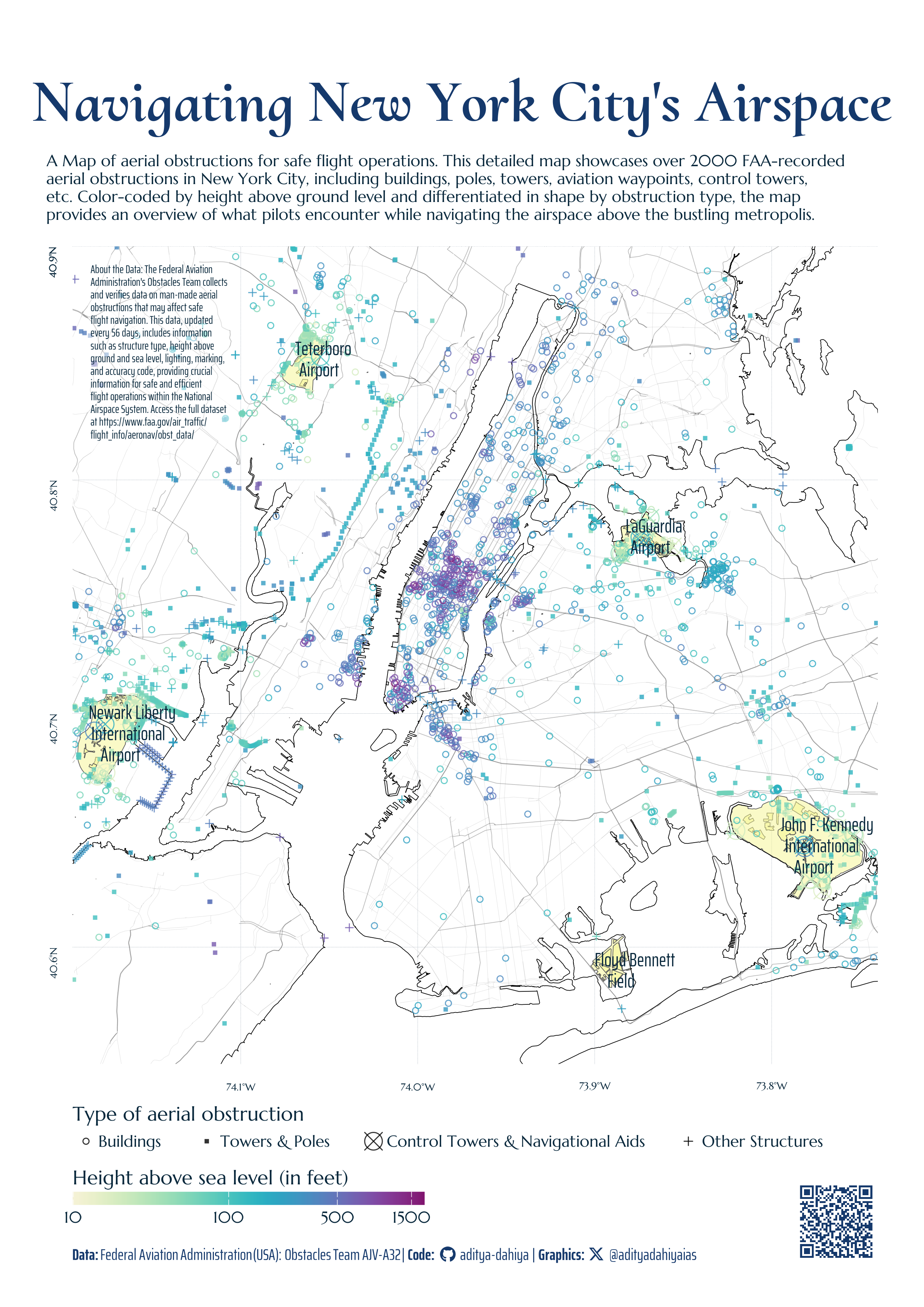
A map showcasing over 2000 FAA-recorded aerial obstructions in New York City, including buildings, poles, towers, aviation waypoints, control towers, etc. Color-coded by height above ground level and differentiated in shape by obstruction type, the map provides an overview of what pilots encounter while navigating the airspace above the bustling metropolis.

The detailed Figure 1 showcases over 2000 FAA-recorded aerial obstructions in and around New York City! This map provides an overview of the city’s skies for safe flight operations, including buildings, poles, towers, aviation waypoints, and control towers. Color-coded by height above ground level and differentiated by obstruction type, it offers a view of the airspace above this bustling metropolis, as seen by Pilots. The data, is updated every 56 days by the Federal Aviation Administration’s Obstacles Team to ensure safe and efficient flight operations within the National Airspace System in USA. Access the full dataset here.

Figure 1: A Map of aerial obstructions for safe flight operations.

How I made this graphic?

Loading required libraries, data import & creating custom functions. The Document for Meta Data, Variable Names and Explanations can be viewed here.

# Data Import and Wrangling Tools
library(tidyverse)            # All things tidy
library(janitor)              # Cleaning names etc.
library(here)                 # Root Directory Management
library(dataverse)            # Getting data from Harvard Dataverse

# Final plot tools
library(scales)               # Nice Scales for ggplot2
library(fontawesome)          # Icons display in ggplot2
library(ggtext)               # Markdown text support for ggplot2
library(showtext)             # Display fonts in ggplot2
library(colorspace)           # Lighten and Darken colours
library(ggthemes)             # Themes for ggplot2
library(patchwork)            # Combining plots

# Mapping tools
library(sf)                   # All spatial objects in R

# Importing raw data
zip_url <- "https://aeronav.faa.gov/Obst_Data/DAILY_DOF_CSV.ZIP"

# Define a temporary file path to save the zip file
temp_zip <- tempfile(fileext = ".zip")
# Download the zip file
download.file(zip_url, temp_zip, mode = "wb")
# Extract the CSV file from the zip
csv_file <- unzip(temp_zip, files = NULL)
# Load the CSV file into R
rawdf <- read_csv(csv_file)
unlink(temp_zip)
unlink("DOF.csv")
rm(csv_file, temp_zip, zip_url)

# Create a function to draw a bounding box to remove features outside it
geometric_rectangle <- function(lat_min, lat_max, lon_min, lon_max) {
  box_coords <- matrix(
    data = c(
      c(lon_min, lon_max, lon_max, lon_min, lon_min),
      c(lat_min, lat_min, lat_max, lat_max, lat_min)
    ),
    ncol = 2, byrow = FALSE
  )
  return(
    st_polygon(list(box_coords)) |> 
      st_sfc(crs = 4326)   # Set the CRS to EPSG:4326, the default
  )
} 

Get New York City Map Data

library(osmdata)

# Bounding Box (Latitude and Longitude limits) for New York City Area
nyc_bbox <- c(-74.195, 40.55, -73.74, 40.9)

# A rectangle to draw around the New York City
nyc_rect <- geometric_rectangle(nyc_bbox[2], nyc_bbox[4],
                                nyc_bbox[1], nyc_bbox[3])

# Data to add Pointers for the main airports
com_airports <- tibble(
  airport = c("John F. Kennedy International Airport",
              "Newark Liberty International Airport",
              "LaGuardia Airport",
              "Long Island MacArthur Airport",
              "Stewart International Airport",
              "Trenton–Mercer Airport",
              "Floyd Bennett Field",
              "Teterboro Airport"),
  lon = c(-73.7817205, -74.17369618, -73.87422493,
          -73.0974269, -74.10118458, -74.81378462,
          -73.8886878, -74.06131113),
  lat = c(40.6433708, 40.69135938, 40.77570745,
          40.7980748, 41.49799333, 40.27745111,
          40.5899426, 40.85165153)
) |> 
  st_as_sf(coords = c("lon", "lat"), crs = 4326)

# Getting NYC streets data
nyc_roads <- opq(bbox = nyc_bbox) |> 
  add_osm_feature(key = "highway", 
                  value = c("motoryway", "trunk",
                            "primary", "secondary")) |> 
  osmdata_sf()

# Getting NYC Airports Data
nyc_air <- opq(bbox = nyc_bbox) |> 
  add_osm_feature(key = "aeroway") |> 
  osmdata_sf()

# Getting Administrative Boundaries of NYC
nyc_boundary <- opq(bbox = nyc_bbox) |> 
  add_osm_feature(key = "boundary", 
                  value = "administrative") |> 
  osmdata_sf()

# Getting NYC Coastline
nyc_coastline <- opq(bbox = nyc_bbox) |> 
  add_osm_feature(key = "natural", 
                  value = "coastline") |> 
  osmdata_sf()

Visualization Parameters

# Font for titles
font_add_google("Cormorant Upright",
  family = "title_font"
) 

# Font for the caption
font_add_google("Saira Extra Condensed",
  family = "caption_font"
) 

# Font for plot text
font_add_google("Marcellus",
  family = "body_font"
) 

showtext_auto()

# Background Colour
bg_col <- "white"

# Colour for the text using FAA's offical website colour
text_col <- "#09283c"  

# Colour for highlighted text
text_hil <- "#15396c"

# Define Base Text Size
ts <- 40 

# Caption stuff for the plot
sysfonts::font_add(
  family = "Font Awesome 6 Brands",
  regular = here::here("docs", "Font Awesome 6 Brands-Regular-400.otf")
)
github <- "&#xf09b"
github_username <- "aditya-dahiya"
xtwitter <- "&#xe61b"
xtwitter_username <- "@adityadahiyaias"
social_caption_1 <- glue::glue("<span style='font-family:\"Font Awesome 6 Brands\";'>{github};</span> <span style='color: {text_hil}'>{github_username}  </span>")
social_caption_2 <- glue::glue("<span style='font-family:\"Font Awesome 6 Brands\";'>{xtwitter};</span> <span style='color: {text_hil}'>{xtwitter_username}</span>")

Plot Text

plot_title <- "Navigating New York City's Airspace"

plot_caption <- paste0(
  "**Data:** Federal Aviation Administration (USA): Obstacles Team AJV-A32", 
  " |  **Code:** ", 
  social_caption_1, 
  " |  **Graphics:** ", 
  social_caption_2
  )

subtitle_text <- "A Map of aerial obstructions for safe flight operations. This detailed map showcases over 2000 FAA-recorded aerial obstructions in New York City, including buildings, poles, towers, aviation waypoints, control towers, etc. Color-coded by height above ground level and differentiated in shape by obstruction type, the map provides an overview of what pilots encounter while navigating the airspace above the bustling metropolis."
plot_subtitle <- str_wrap(subtitle_text, width = 110)
plot_subtitle |> str_view()

text_annotation_1 <- "About the Data: The Federal Aviation Administration's Obstacles Team collects and verifies data on man-made aerial obstructions that may affect safe flight navigation. This data, updated every 56 days, includes information such as structure type, height above ground and sea level, lighting, marking, and accuracy code, providing crucial information for safe and efficient flight operations within the National Airspace System. Access the full dataset at https://www.faa.gov/air_traffic/flight_info/aeronav/obst_data/"

Data Analysis and Wrangling

# Air Obstacles in New York City
nyc_arobs <- rawdf |> 
  clean_names() |> 
  mutate(
    agl = as.numeric(agl),
    amsl = as.numeric(amsl)
  ) |> 
  filter(latdec > nyc_bbox[2] & latdec < nyc_bbox[4]) |> 
  filter(londec > nyc_bbox[1] & londec < nyc_bbox[3]) |> 
  mutate(
    type = case_when(
      type %in% c("BLDG", "BLDG-TWR") ~ "Buildings",
      type %in% c("TOWER", "POLE", "T-L TWR", 
                  "UTILITY POLE", "ANTENNA") ~ "Towers & Poles",
      type %in% c("CTRL TWR", 
                  "NAVAID") ~ "Control Towers & Navigational Aids",
      .default = "Other Structures"
    ),
    type = fct(type, levels = c(
      "Buildings",
      "Towers & Poles",
      "Control Towers & Navigational Aids",
      "Other Structures"
    ))
  ) |> 
  select(oas, state, city, lat = latdec, lon = londec,
         type, agl, amsl) |> 
  st_as_sf(coords = c("lon", "lat"), crs = 4326)

NYC Aerial Obstructions plot

g_base <- ggplot() +
  
  # Outer Rectangle of the map
  # geom_sf(
  #   data = nyc_rect,
  #   colour = text_col,
  #   linewidth = 1, 
  #   linetype = 1
  # ) +
  
  # Airports of NYC
  geom_sf(
    data = nyc_air$osm_polygons,
    fill = "#f5f590",
    alpha = 0.5
  ) +
  
  # Coastline of New York City and surrounding areas
  geom_sf(
    data = nyc_coastline$osm_lines,
    linewidth = 0.2,
    linetype = 1
  ) +
  
  # Plotting major roads of New York Cities
  geom_sf(
    data = nyc_roads$osm_lines |> 
            filter(highway %in% c(
              "motorway", "trunk", "primary"
            )),
    colour = "grey10",
    alpha = 0.3,
    linewidth = 0.2,
    linetype = 1
  ) +
  
  # Plotting minor roads of New York Cities
  geom_sf(
    data = nyc_roads$osm_lines |> 
            filter(highway == "secondary"),
    colour = "grey10",
    alpha = 0.15,
    linewidth = 0.1,
    linetype = 1
  ) +
  
  # Plotting the Aerial Obstructions
  geom_sf(
    data = nyc_arobs,
    mapping = aes(
      colour = amsl,
      shape = type,
      size = type
    ),
    alpha = 0.8
  ) +
  
  # Add names of the major airports
  geom_sf_text(
    data = com_airports,
    mapping = aes(label = str_wrap(airport, 15)),
    lineheight = 0.3,
    family = "caption_font",
    face = "bold",
    colour = text_col,
    size = ts / 3,
    hjust = 0.25,
    vjust = 0.5
  ) +

  # Colour, shape and size scales
  paletteer::scale_colour_paletteer_c(
    # "ggthemes::Red-Gold",
    # "ggthemes::Classic Red",
    # "grDevices::Purple-Blue",
    "grDevices::Purple-Yellow",
    # "grDevices::Plasma",
    # "grDevices::Mako",
    # "grDevices::ag_Sunset",
    direction = -1,
    name = "Height above sea level (in feet)",
    trans = "log2",
    breaks = c(0, 10, 100, 500, 1500)
  ) +
  scale_shape_manual(
    name = "Type of aerial obstruction",
    values = c(1, 15, 13, 3)
  ) +
  scale_size_manual(
    name = "Type of aerial obstruction",
    values = c(1.5, 1, 5, 1.5)
  ) +
  scale_y_continuous(
    breaks = seq(40.6, 40.9, 0.1)
  ) +
  scale_x_continuous(
    position = "top"
  ) +
  guides(
    colour = guide_colourbar(
      theme = theme(
        legend.key.width = unit(80, "mm"),
        legend.key.height = unit(3, "mm"),
        legend.text = element_text(
          colour = text_col, 
          margin = margin(1, 0, 1, 0, "mm"),
          vjust = 0.5
        )
      )
    )
  ) +
  
  # Coordinates and limits for the plot
  coord_sf(
    expand = FALSE, 
    xlim = c(nyc_bbox[1], nyc_bbox[3]),
    ylim = c(nyc_bbox[2], nyc_bbox[4])
  ) +
  
  # Lables and Annotations
  labs(
    title = plot_title,
    subtitle = plot_subtitle,
    caption = plot_caption,
    x = NULL, y = NULL
  ) +
  
  # Themes
  theme_minimal(
    base_size = ts,
    base_family = "body_font"
  ) +
  theme(
    legend.position = "bottom",
    legend.direction = "horizontal",
    legend.box = "vertical",
    legend.margin = margin(0,0,0,0, "mm"),
    legend.spacing = unit(0, "mm"),
    legend.title.position = "top",
    legend.box.just = "left",
    legend.justification = "left",
    legend.background = element_rect(fill = NA, colour = NA),
    legend.box.background = element_rect(fill = NA, colour = NA),
    legend.box.spacing = unit(0, "mm"),
    legend.box.margin = margin(0, 0, 0, 0, "mm"),
    legend.text = element_text(
      colour = text_col, 
      margin = margin(0, 0, 0, 0, "mm"),
      vjust = 0.5
    ),
    legend.title = element_text(
      size = ts,
      colour = text_col,
      margin = margin(3, 0, 1, 0, "mm")
    ),
    axis.text.y = element_text(
      margin = margin(0,0,0,0, "mm"),
      colour = text_col,
      size = ts / 2,
      angle = 90, 
      hjust = 1, 
      vjust = 0
    ),
    axis.text.x = element_text(
      margin = margin(0,0,0,0, "mm"),
      colour = text_col,
      size = ts / 2, 
      vjust = 0,
      hjust = 0.5
    ),
    panel.grid = element_line(
      colour = text_col |> lighten(0.5),
      linewidth = 0.1,
      linetype = 3
    ),
    axis.ticks = element_blank(),
    axis.title = element_blank(),
    axis.line = element_blank()
  ) +
  theme(
    plot.background = element_rect(
      fill = bg_col,
      linewidth = NA, 
      colour = NA
    ),
    plot.title = element_text(
      size = 3 * ts,
      face = "bold",
      colour = text_hil,
      family = "title_font",
      margin = margin(10, 0, 2, 0,"mm"),
      hjust = 0.5
    ),
    plot.subtitle = element_text(
      hjust = 0, 
      lineheight = 0.3,
      colour = text_col,
      family = "body_font",
      margin = margin(2, 0, 5, 0, "mm"),
      size = 0.8 * ts
    ),
    plot.caption = ggtext::element_textbox(
      hjust = 0,
      family = "caption_font",
      colour = text_hil,
      margin = margin(4, 0, 1, 0, "mm")
    ), 
    plot.title.position = "plot"
  )

Add-on maps, insets and annotations

g2 <- ggplot() +
  annotate(
    geom = "label",
    x = 0,
    y = 0,
    label = str_wrap(
      text_annotation_1,
      width = 40,
      whitespace_only = F
      ),
    lineheight = 0.3,
    size = ts / 5,
    fill = bg_col,
    alpha = 0.5,
    colour = text_col,
    label.size = NA,
    family = "caption_font",
    hjust = 0
  ) + 
  theme_void()

# QR Code for the plot
url_graphics <- paste0(
  "https://aditya-dahiya.github.io/projects_presentations/data_vizs/",
  # The file name of the current .qmd file
  "nyc_air_obstacles",         
  ".html"
)
# remotes::install_github('coolbutuseless/ggqr')
# library(ggqr)
plot_qr <- ggplot(
  data = NULL, 
  aes(x = 0, y = 0, label = url_graphics)
  ) + 
  ggqr::geom_qr(
    colour = text_hil, 
    fill = bg_col,
    size = 0.65
    ) +
  coord_fixed() +
  theme_void() +
  theme(plot.background = element_rect(
    fill = NA, 
    colour = NA
    )
  )

Compiling Plots with Patchwork

g <- g_base +
  
  # Add inset to the plot
  inset_element(
    p = g2, 
    left = -0.12, 
    right = 0.22,
    bottom = 0.75,
    top = 1, 
    align_to = "plot",
    clip = TRUE
  ) +
  
  # Add QR Code to the plot
  inset_element(
    p = plot_qr, 
    left = 0.9, 
    right = 1,
    bottom = -0.33,
    top = 0.02, 
    align_to = "plot",
    clip = TRUE
  ) +
  
  # Basix Plot Annotations
  plot_annotation(
    theme = theme(
      plot.background = element_rect(
        fill = bg_col, 
        colour = NA, 
        linewidth = 0
      )
    )
  )

Savings the graphics

ggsave(
  filename = here::here("data_vizs", "nyc_air_obstacles.png"),
  plot = g,
  width = 210,    # Default A4 size page
  height = 297,   # Default A4 size page
  units = "mm",
  bg = bg_col
)


library(magick)
# Saving a thumbnail for the webpage
image_read(here::here("data_vizs", "nyc_air_obstacles.png")) |> 
  image_resize(geometry = "400") |> 
  image_write(here::here("data_vizs", "thumbnails", "nyc_air_obstacles.png"))