Who’s the Reference? Racial Patterns in studies.

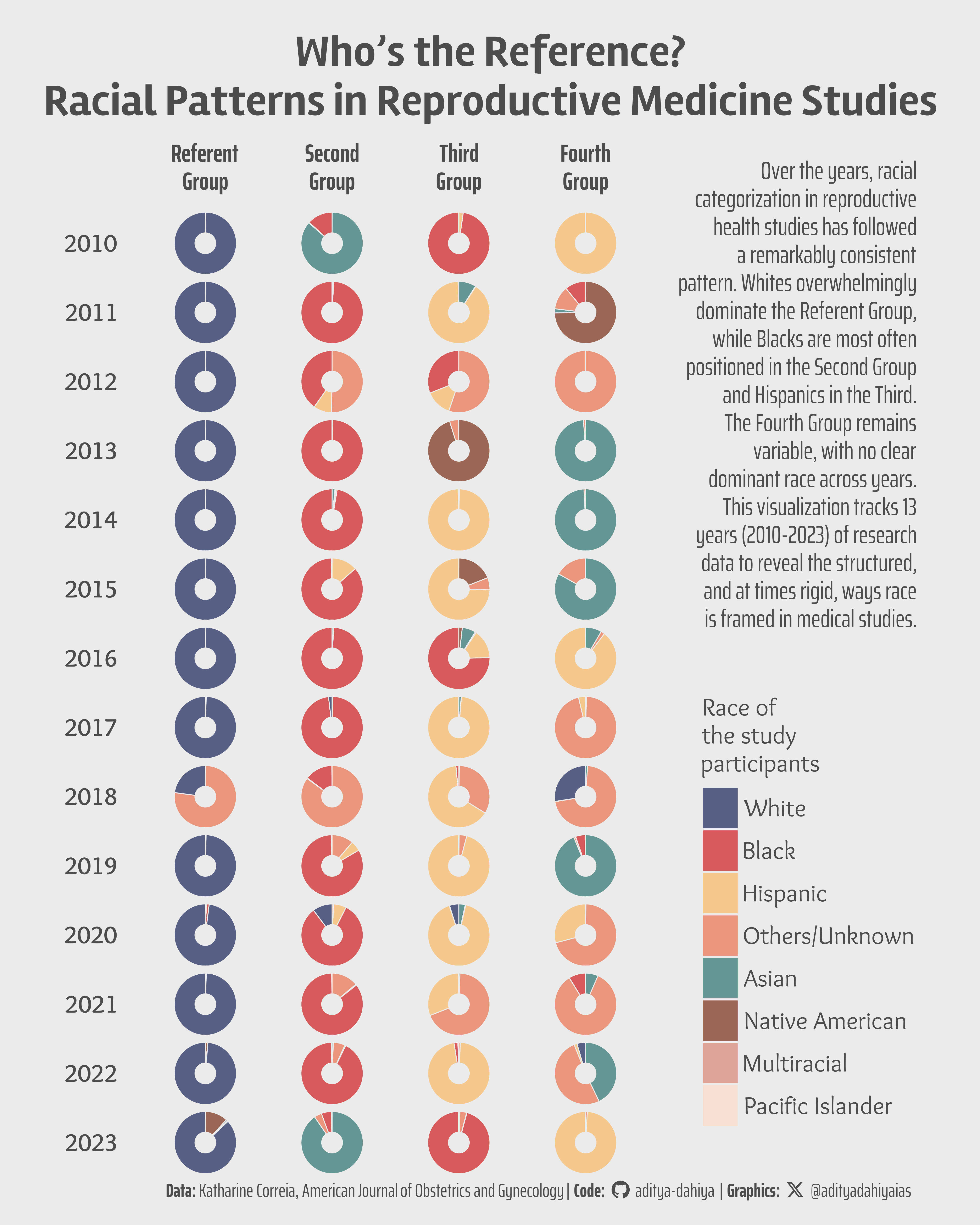
Over the years, racial categorization in reproductive health studies has followed a remarkably consistent pattern. Whites overwhelmingly dominate the Referent Group, while Blacks are most often positioned in the Second Group and Hispanics in the Third. The Fourth Group remains variable, with no clear dominant race across years. This visualization tracks 13 years (2010-2023) of research data to reveal the structured, and at times rigid, ways race is framed in medical studies.

About the Data

This dataset compiles information from academic literature on racial and ethnic disparities in reproductive medicine, focusing on studies published in the eight highest-impact peer-reviewed Ob/Gyn journals from January 2010 to June 2023. The data were collected for a review article, Racial and ethnic disparities in reproductive medicine in the United States, published in the American Journal of Obstetrics and Gynecology. This dataset provides insights into how racial and ethnic disparities are framed, measured, and discussed in the literature, enabling researchers to explore variations in sample sizes, study types, and health outcomes. A companion interactive website accompanies the dataset, offering dynamic exploration tools.

This dataset has also inspired creative awareness projects, including data art by students.

Figure 1: Each facet in this grid represents a year from 2010 to 2023, with four horizontally arranged groups—Referent Group, Second Group, Third Group, and Fourth Group—reflecting how racial categories are structured in research studies. Within each facet, the donut charts show the racial composition of each group, with different colors representing distinct racial categories. The size of each segment corresponds to the proportion of individuals from that racial category in a given group. This visualization highlights how race has been classified over time in reproductive health research.

How I made this graphic?

Loading required libraries

# Data Import and Wrangling Tools
library(tidyverse)            # All things tidy

# Final plot tools
library(scales)               # Nice Scales for ggplot2
library(fontawesome)          # Icons display in ggplot2
library(ggtext)               # Markdown text support for ggplot2
library(showtext)             # Display fonts in ggplot2
library(colorspace)           # Lighten and Darken colours

# Getting data
article_dat <- readr::read_csv('https://raw.githubusercontent.com/rfordatascience/tidytuesday/main/data/2025/2025-02-25/article_dat.csv')
model_dat <- readr::read_csv('https://raw.githubusercontent.com/rfordatascience/tidytuesday/main/data/2025/2025-02-25/model_dat.csv')

Visualization Parameters

# Font for titles
font_add_google("Rambla",
  family = "title_font"
) 

# Font for the caption
font_add_google("Saira Extra Condensed",
  family = "caption_font"
) 

# Font for plot text
font_add_google("Overlock",
  family = "body_font"
) 

showtext_auto()

# A base Colour
bg_col <- "grey92"
seecolor::print_color(bg_col)

# Colour for highlighted text
text_hil <- "grey30"
seecolor::print_color(text_hil)

# Colour for the text
text_col <- "grey30"
seecolor::print_color(text_col)

# Define Base Text Size
bts <- 90 

# Caption stuff for the plot
sysfonts::font_add(
  family = "Font Awesome 6 Brands",
  regular = here::here("docs", "Font Awesome 6 Brands-Regular-400.otf")
)
github <- "&#xf09b"
github_username <- "aditya-dahiya"
xtwitter <- "&#xe61b"
xtwitter_username <- "@adityadahiyaias"
social_caption_1 <- glue::glue("<span style='font-family:\"Font Awesome 6 Brands\";'>{github};</span> <span style='color: {text_hil}'>{github_username}  </span>")
social_caption_2 <- glue::glue("<span style='font-family:\"Font Awesome 6 Brands\";'>{xtwitter};</span> <span style='color: {text_hil}'>{xtwitter_username}</span>")
plot_caption <- paste0(
  "**Data:** Katharine Correia, American Journal of Obstetrics and Gynecology", 
  " |  **Code:** ", 
  social_caption_1, 
  " |  **Graphics:** ", 
  social_caption_2
  )
rm(github, github_username, xtwitter, 
   xtwitter_username, social_caption_1, 
   social_caption_2)

# Add text to plot-------------------------------------------------
plot_title <- "Who’s the Reference?\nRacial Patterns in Reproductive Medicine Studies"

plot_subtitle <- str_wrap("Over the years, racial categorization in reproductive health studies has followed a remarkably consistent pattern. Whites overwhelmingly dominate the Referent Group, while Blacks are most often positioned in the Second Group and Hispanics in the Third. The Fourth Group remains variable, with no clear dominant race across years. This visualization tracks 13 years (2010-2023) of research data to reveal the structured, and at times rigid, ways race is framed in medical studies.", 30)

str_view(plot_subtitle)

Exploratory Data Analysis and Wrangling

# library(summarytools)
# article_dat |> 
#   dfSummary() |> 
#   view()

# Helper function to recategorize race variables
recode_race <- function(x) {
  case_when(
    x %in% c("White", "white", "Non-Hispanic White",
             "Non-Hispanic white", "Caucasian",
             "non-Hispanic white", "White, non-Hispanic",
             "non-Hispanic White", "White non-Hispanic",
             "White/Caucasian", "Whites", "Non Hispanic white",
             "Non-Hispanic, White", "Non Hispanic whites",
             "Caucasian/White") ~ "White",
    
    x %in% c("Black", "African American",
             "Non-Hispanic Black", "Black or African American",
             "Non-Hispanic black", "African American or Black",
             "African American, non-Hispanic", "Black, non-Hispanic",
             "Non Hispanic Black") ~ "Black",
    
    x %in% c("Hispanic", "Latino", "Latina",
             "Hispanic/Latino", "Hispanic/Latina",
             "Hispanic or Latino", "Latinx") ~ "Hispanic",
    
    x %in% c("Asian", "Asian, non-Hispanic",
             "East Asian", "South Asian", "Southeast Asian",
             "Asian American", "Asian, not Hispanic",
             "Asian/Pacific Islander") ~ "Asian",
    
    x %in% c("American Indian", "American Indian/Alaska Native",
             "American Indian/Alaskan", 
             "American Indian/Alaskan Native",
             "Indigenous", "Native American") ~ "Native American",
    
    x %in% c("Pacific Islander", "Native Hawaiian",
             "Native Hawaiian or Other Pacific Islander",
             "Pacific Islander/Native Hawaiian",
             "Other Pacific Islander") ~ "Pacific Islander",
    
    x %in% c("Multiracial", "Two or More Races",
             "Mixed Race", "More than one race",
             "Mixed", "Multiple races") ~ "Multiracial",
    
    is.na(x) | x %in% c("", "Unknown", "Other", "N/A") ~ "Others/Unknown",
    
    TRUE ~ "Others/Unknown"
  )
}

df1 <- article_dat |> 
  select(journal, year, study_type, 
         race1, race1_ss, race2, race2_ss, 
         race3, race3_ss, race4, race4_ss) |> 
  mutate(
    race1 = recode_race(race1),
    race2 = recode_race(race2),
    race3 = recode_race(race3),
    race4 = recode_race(race4)
  )


  # mutate(study_type = case_when(
  #   study_type %in% c("Case-control") ~ "Case-Control",
  #   study_type %in% c("Cross-Sectional", "Cross-sectional") ~ "Cross-Sectional",
  #   study_type %in% c("Prospective Cohort", "Prospective cohort") ~ "Prospective Cohort",
  #   study_type %in% c("Retrospective Cohort", "Retrospective cohort") ~ "Retrospective Cohort",
  #   study_type %in% c("RCT") ~ "Randomized Controlled Trial",
  #   study_type %in% c("Registry") ~ "Registry",
  #   is.na(study_type) ~ "Missing",
  #   TRUE ~ study_type  # Keep any other values unchanged
  # ))


df2 <- bind_rows(
  df1 |> 
    group_by(year, race1) |> 
    summarise(
      count = sum(race1_ss, na.rm = T)
    ) |> 
    group_by(year) |> 
    mutate(
      prop = count / sum(count),
      race = race1,
      type = "Referent\nGroup"
    ) |> 
    select(-race1),
  
  df1 |> 
    group_by(year, race2) |> 
    summarise(
      count = sum(race2_ss, na.rm = T)
    ) |> 
    group_by(year) |> 
    mutate(
      prop = count / sum(count),
      race = race2,
      type = "Second\nGroup"
    ) |> 
    select(-race2),

  df1 |> 
    group_by(year, race3) |> 
    summarise(
      count = sum(race3_ss, na.rm = T)
    ) |> 
    group_by(year) |> 
    mutate(
      prop = count / sum(count),
      race = race3,
      type = "Third\nGroup"
    ) |> 
    select(-race3),

  df1 |> 
    group_by(year, race4) |> 
    summarise(
      count = sum(race4_ss, na.rm = T)
    ) |> 
    group_by(year) |> 
    mutate(
      prop = count / sum(count),
      race = race4,
      type = "Fourth\nGroup"
    ) |> 
    select(-race4)
) |> 
  mutate(
    type = fct(
      type,
      levels = c("Referent\nGroup", "Second\nGroup",
                 "Third\nGroup", "Fourth\nGroup")
    )
  ) |> 
  ungroup()

race_levels <- df2 |> 
  count(race, wt = count, sort = T) |> 
  pull(race)

df3 <- df2 |> 
  mutate(race = fct(race, levels = race_levels))

The Base Plots

g <- df3 |> 
  ggplot(
    mapping = aes(
      x = 1,
      y = prop,
      fill = race
    )
  ) +
  geom_col(
    colour = bg_col,
    width = 0.4
  ) +
  scale_x_continuous(
    limits = c(0.6, 1.2),
    expand = expansion(0)
  ) +
  paletteer::scale_fill_paletteer_d(
    "tvthemes::Day",
    direction = -1
  ) +
  coord_polar(
    theta = "y",
    clip = "off"
  ) +
  facet_grid(year~type, switch = "y") +
  
  labs(
    x = NULL,
    y = NULL,
    colour = NULL,
    subtitle = plot_subtitle,
    title = plot_title,
    caption = plot_caption,
    fill = "Race of\nthe study\nparticipants"
  ) +
  theme_minimal(
    base_family = "body_font",
    base_size = bts
  ) +
  theme(
    
    # Overall Plot
    plot.title.position = "plot",
    text = element_text(
      margin = margin(0,0,0,0, "mm"),
      colour = text_hil,
      hjust = 0.5,
      vjust = 0.5
    ),
    plot.title = element_text(
        margin = margin(0,0,15,0, "mm"),
        colour = text_hil,
        hjust = 0.5,
        size = bts * 1.75,
        family = "title_font",
        face = "bold",
        lineheight = 0.3
      ),
    plot.subtitle = element_text(
      colour = text_hil,
      size = bts,
      hjust = 1, 
      vjust = 1,
      lineheight = 0.3,
      margin = margin(0,0,-200,0, "mm"),
      family = "caption_font"
    ),
    plot.caption = element_textbox(
      halign = 0,
      hjust = 0,
      family = "caption_font",
      margin = margin(0,0,0,0, "mm"),
      size = 0.75 * bts
    ),
    plot.margin = margin(15,5,10,5, "mm"),
    panel.background = element_rect(
      fill = "transparent",
      colour = "transparent"
    ),
    plot.background = element_rect(
      fill = "transparent",
      colour = "transparent"
    ),
    
    # Axis and Strips
    axis.text = element_blank(),
    axis.ticks = element_blank(),
    axis.ticks.length = unit(0, "mm"),
    panel.spacing.y = unit(-3.5, "mm"),
    panel.spacing.x = unit(20, "mm"),
    strip.text.x = element_text(
      margin = margin(0,0,5,0, "mm"),
      angle = 0,
      face = "bold",
      family = "caption_font",
      size = bts,
      lineheight = 0.3,
      colour = text_col
    ),
    strip.text.y.left = element_text(
      angle = 0,
      margin = margin(0,20,0,0, "mm"),
      face = "bold",
      size = bts,
      colour = text_col
    ),
    
    # Legend
    legend.position = "right",
    legend.justification = c(1, 0.1),
    legend.text = element_text(
      margin = margin(4,0,4,2, "mm"),
      size = bts
    ),
    legend.key.height = unit(5, "mm"),
    legend.key.width = unit(15, "mm"),
    legend.margin = margin(0,0,0,0, "mm"),
    legend.box.margin = margin(0,0,0,0, "mm"),
    legend.title = element_text(
      lineheight = 0.3,
      margin = margin(0,0,5,0, "mm")
    )
    
  )

ggsave(
  filename = here::here(
    "data_vizs",
    "tidy_acad_lit_med.png"
  ),
  plot = g,
  width = 400,
  height = 500,
  units = "mm",
  bg = bg_col
)

Savings the thumbnail for the webpage

# Saving a thumbnail

library(magick)

# Saving a thumbnail for the webpage
image_read(here::here("data_vizs", 
                      "tidy_acad_lit_med.png")) |> 
  image_resize(geometry = "x400") |> 
  image_write(
    here::here(
      "data_vizs", 
      "thumbnails", 
      "tidy_acad_lit_med.png"
    )
  )

Session Info

# Data Import and Wrangling Tools
library(tidyverse)            # All things tidy

# Final plot tools
library(scales)               # Nice Scales for ggplot2
library(fontawesome)          # Icons display in ggplot2
library(ggtext)               # Markdown text support for ggplot2
library(showtext)             # Display fonts in ggplot2
library(colorspace)           # Lighten and Darken colours

sessioninfo::session_info()$packages |> 
  as_tibble() |> 
  select(package, 
         version = loadedversion, 
         date, source) |> 
  arrange(package) |> 
  janitor::clean_names(
    case = "title"
  ) |> 
  gt::gt() |> 
  gt::opt_interactive(
    use_search = TRUE
  ) |> 
  gtExtras::gt_theme_espn()

Table 1: R Packages and their versions used in the creation of this page and graphics