Created with ggplot2 + coord_polar() for pie charts, ggflags for country indicators, showtext for custom fonts, and scales for proportional sizing based on average calories per recipe
#TidyTuesday
Author
Aditya Dahiya
Published
September 23, 2025
About the Data
This week’s dataset explores a comprehensive collection of recipes from Allrecipes.com, curated through the tastyR package and prepared for analysis. The collection includes two complementary datasets: all_recipes containing 14,426 general recipes, and cuisines featuring 2,218 recipes categorized by country of origin. Both datasets provide rich recipe information including ingredients, comprehensive nutritional data (calories, fat, carbohydrates, protein), cooking logistics (preparation and cooking times), user engagement metrics (ratings and reviews), and serving sizes. All data has been systematically cleaned and standardized to facilitate straightforward comparisons and visual exploration. The datasets open up numerous analytical opportunities, from identifying the most successful recipe authors and exploring relationships between cooking time and ratings, to discovering which cuisines achieve the highest user satisfaction and finding the most “actionable” recipes that balance high ratings with minimal time investment. This curated collection was assembled by Brian Mubia and represents a valuable resource for exploring culinary trends, user preferences, and recipe performance patterns across diverse cooking traditions and styles.
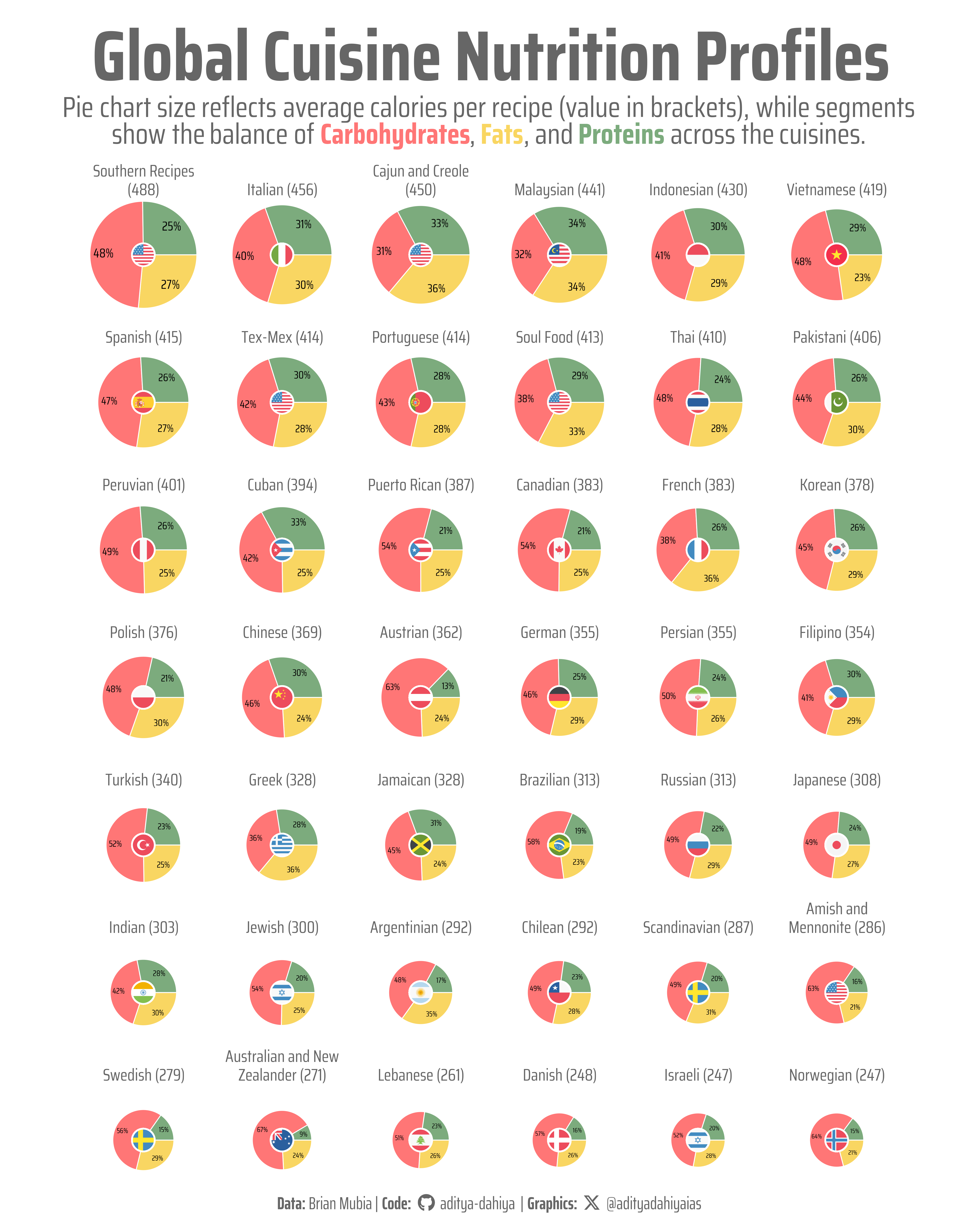
Figure 1: This visualization explores the nutritional profiles of 42 global cuisines from the Allrecipes dataset, with each pie chart representing a different culinary tradition. The size of each pie is proportional to the average calories per recipe, ranging from Malaysian cuisine at 247 calories to Italian at 488 calories. Within each pie, colored segments reveal the macronutrient balance: red for carbohydrates, yellow for fats, and green for proteins, with percentages displayed for each segment. Country flags at the center help identify each cuisine’s origin. The data reveals fascinating patterns—Italian and German cuisines tend to be more calorie-dense, while Asian cuisines like Vietnamese and Thai generally show lower calorie averages. Some cuisines like Brazilian and Turkish show relatively balanced macronutrient distributions, while others like certain European cuisines lean more heavily toward carbohydrates, reflecting their traditional grain and pasta-based dishes.
How I Made This Graphic
I created this comprehensive visualization using R and the tidyverse ecosystem, leveraging several specialized packages for enhanced functionality. The foundation was built with ggplot2 for the core plotting framework, enhanced by ggtext for markdown text support in titles and subtitles. I used showtext and Google Fonts to incorporate custom typography (Saira family fonts) for a polished aesthetic. The polar coordinate system transformed rectangular bar charts into pie charts using coord_polar(), while ggflags added country flags at each pie center. Data manipulation relied heavily on dplyr for grouping and summarizing nutritional data, with tidyr for reshaping data into the long format required for visualization. The scales package normalized calorie values to create proportional pie sizes, and patchwork enabled the multi-panel layout through facet_wrap(). Color choices used a custom palette to distinguish carbohydrates, fats, and proteins across the 42 featured cuisines.
Loading required libraries
Code
pacman::p_load( tidyverse, # All things tidy scales, # Nice Scales for ggplot2 fontawesome, # Icons display in ggplot2 ggtext, # Markdown text support for ggplot2 showtext, # Display fonts in ggplot2 colorspace, # Lighten and Darken colours patchwork # Composing Plots)all_recipes <- readr::read_csv('https://raw.githubusercontent.com/rfordatascience/tidytuesday/main/data/2025/2025-09-16/all_recipes.csv')cuisines <- readr::read_csv('https://raw.githubusercontent.com/rfordatascience/tidytuesday/main/data/2025/2025-09-16/cuisines.csv')# Source: Claude Sonnet 4.0# Create a tibble mapping cuisines to their primary country ISO-2 codeslibrary(tibble)cuisine_country_mapping <-tibble(country =c("Southern Recipes", "Italian", "Cajun and Creole", "Malaysian", "Indonesian", "Vietnamese", "Spanish", "Tex-Mex", "Portuguese", "Soul Food", "Thai", "Pakistani", "Peruvian", "Cuban", "Puerto Rican", "Canadian", "French", "Korean", "Polish", "Chinese", "Austrian", "German", "Persian", "Filipino", "Turkish", "Greek", "Jamaican", "Brazilian", "Russian", "Japanese", "Indian", "Jewish", "Argentinian", "Chilean", "Scandinavian", "Amish and Mennonite", "Swedish", "Australian and New Zealander", "Lebanese", "Danish", "Israeli", "Norwegian" ),country_code =c("us", # Southern Recipes - United States (Southern US cuisine)"it", # Italian - Italy"us", # Cajun and Creole - United States (Louisiana)"my", # Malaysian - Malaysia"id", # Indonesian - Indonesia"vn", # Vietnamese - Vietnam"es", # Spanish - Spain"us", # Tex-Mex - United States (Texas-Mexico border cuisine)"pt", # Portuguese - Portugal"us", # Soul Food - United States (African-American cuisine)"th", # Thai - Thailand"pk", # Pakistani - Pakistan"pe", # Peruvian - Peru"cu", # Cuban - Cuba"pr", # Puerto Rican - Puerto Rico"ca", # Canadian - Canada"fr", # French - France"kr", # Korean - South Korea"pl", # Polish - Poland"cn", # Chinese - China"at", # Austrian - Austria"de", # German - Germany"ir", # Persian - Iran"ph", # Filipino - Philippines"tr", # Turkish - Turkey"gr", # Greek - Greece"jm", # Jamaican - Jamaica"br", # Brazilian - Brazil"ru", # Russian - Russia"jp", # Japanese - Japan"in", # Indian - India"il", # Jewish - Israel (modern Jewish cuisine center)"ar", # Argentinian - Argentina"cl", # Chilean - Chile"se", # Scandinavian - Sweden (largest Scandinavian country)"us", # Amish and Mennonite - United States (primarily Pennsylvania)"se", # Swedish - Sweden"au", # Australian and New Zealander - Australia (larger population)"lb", # Lebanese - Lebanon"dk", # Danish - Denmark"il", # Israeli - Israel"no"# Norwegian - Norway ))
Visualization Parameters
Code
# Font for titlesfont_add_google("Saira",family ="title_font")# Font for the captionfont_add_google("Saira Condensed",family ="body_font")# Font for plot textfont_add_google("Saira Extra Condensed",family ="caption_font")showtext_auto()# A base Colourbg_col <-"white"seecolor::print_color(bg_col)# Colour for highlighted texttext_hil <-"grey40"seecolor::print_color(text_hil)# Colour for the texttext_col <-"grey30"seecolor::print_color(text_col)line_col <-"grey30"# Define Base Text Sizebts <-80# Caption stuff for the plotsysfonts::font_add(family ="Font Awesome 6 Brands",regular = here::here("docs", "Font Awesome 6 Brands-Regular-400.otf"))github <-""github_username <-"aditya-dahiya"xtwitter <-""xtwitter_username <-"@adityadahiyaias"social_caption_1 <- glue::glue("<span style='font-family:\"Font Awesome 6 Brands\";'>{github};</span> <span style='color: {text_hil}'>{github_username} </span>")social_caption_2 <- glue::glue("<span style='font-family:\"Font Awesome 6 Brands\";'>{xtwitter};</span> <span style='color: {text_hil}'>{xtwitter_username}</span>")plot_caption <-paste0("**Data:** Brian Mubia"," | **Code:** ", social_caption_1," | **Graphics:** ", social_caption_2)rm( github, github_username, xtwitter, xtwitter_username, social_caption_1, social_caption_2)# Add text to plot-------------------------------------------------plot_title <-"Global Cuisine Nutrition Profiles"plot_subtitle <-"Pie chart size reflects average calories per recipe (value in brackets), while segments<br>show the balance of <b style='color:#FF7676'>**Carbohydrates**</b>, <b style='color:#F9D662'>**Fats**</b>, and <b style='color:#7CAB7D'>**Proteins**</b> across the cuisines."str_view(plot_subtitle)
# Saving a thumbnaillibrary(magick)# Saving a thumbnail for the webpageimage_read(here::here("data_vizs","tidy_allrecipes.png")) |>image_resize(geometry ="x400") |>image_write( here::here("data_vizs","thumbnails","tidy_allrecipes.png" ) )