Amazon’s Hidden Story: What Word Frequency Reveals About Its Journey

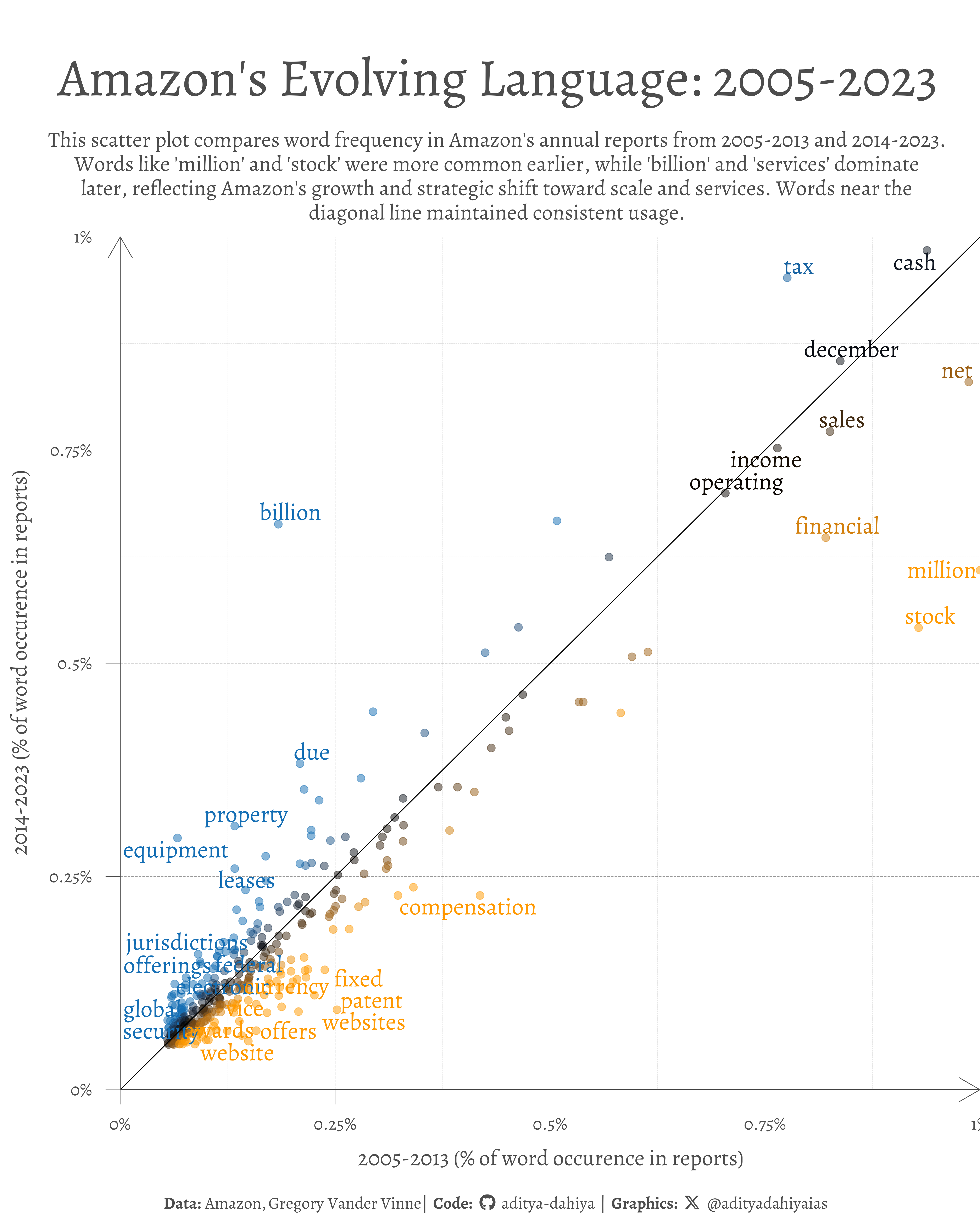
This scatter plot visualizes word frequency in Amazon’s annual reports, comparing two time periods. The x-axis represents the percentage of total words from 2005-2013, while the y-axis shows the same for 2014-2023. Each dot corresponds to a word, and the diagonal line indicates equal usage across both periods.

About the Data

The data for this week’s exploration comes from Amazon’s annual reports, which are released yearly by the publicly-traded company with a December 31st year-end. These reports summarize Amazon’s financial performance, achievements, and challenges over the past year. The dataset, curated by Gregory Vander Vinne, was processed by reading PDFs into R using the {pdftools} R package. It was featured in a TidyTuesday post on Gregory’s website, where stop words like “and” or “the” were removed for cleaner analysis. Participants can access the data via the tidytuesdayR package or directly from GitHub.

This dataset invites exploration of trends like word usage over time, sentiment shifts, and word co-occurrences.

This scatter plot illustrates the evolution of language in Amazon’s annual reports, comparing word frequency between 2005-2013 (x-axis) and 2014-2023 (y-axis). Each point represents a word, with a 45-degree line marking equal usage across both periods. In 2005-2013, terms like “million” and “stock” were prevalent, emphasizing financial metrics. By 2014-2023, “billion” and “services” rose, reflecting growth in scale and services. Deviations from the line reveal shifts in Amazon’s strategic focus.

Figure 1: The graphic displays a scatter plot of word usage in Amazon’s annual reports. The x-axis plots the frequency of words from 2005-2013, and the y-axis plots the frequency from 2014-2023. A 45-degree diagonal line marks where words have consistent frequency between the two eras.

How I made this graphic?

Loading required libraries

# Data Import and Wrangling Tools
library(tidyverse)            # All things tidy

# Final plot tools
library(scales)               # Nice Scales for ggplot2
library(fontawesome)          # Icons display in ggplot2
library(ggtext)               # Markdown text support for ggplot2
library(showtext)             # Display fonts in ggplot2
library(colorspace)           # Lighten and Darken colours
library(tidytext)             # Text Analysis for R
library(ggrepel)              # Text Labels non-overlapping
library(paletteer)            # colour Palettes

report_words_clean <- readr::read_csv('https://raw.githubusercontent.com/rfordatascience/tidytuesday/main/data/2025/2025-03-25/report_words_clean.csv')

Visualization Parameters

# Font for titles
font_add_google("Alegreya",
  family = "title_font"
) 

# Font for the caption
font_add_google("Stint Ultra Condensed",
  family = "caption_font"
) 

# Font for plot text
font_add_google("Alegreya",
  family = "Josefin Slab"
) 

showtext_auto()

mypal <- c("#ff9900", "#146eb4", "#000000")
# cols4all::c4a_gui()

# A base Colour
bg_col <- "white"
seecolor::print_color(bg_col)

# Colour for highlighted text
text_hil <- "grey30"
seecolor::print_color(text_hil)

# Colour for the text
text_col <- "grey30"
seecolor::print_color(text_col)

line_col <- "grey30"

# Define Base Text Size
bts <- 120

# Caption stuff for the plot
sysfonts::font_add(
  family = "Font Awesome 6 Brands",
  regular = here::here("docs", "Font Awesome 6 Brands-Regular-400.otf")
)
github <- "&#xf09b"
github_username <- "aditya-dahiya"
xtwitter <- "&#xe61b"
xtwitter_username <- "@adityadahiyaias"
social_caption_1 <- glue::glue("<span style='font-family:\"Font Awesome 6 Brands\";'>{github};</span> <span style='color: {text_hil}'>{github_username}  </span>")
social_caption_2 <- glue::glue("<span style='font-family:\"Font Awesome 6 Brands\";'>{xtwitter};</span> <span style='color: {text_hil}'>{xtwitter_username}</span>")
plot_caption <- paste0(
  "**Data:** Amazon, Gregory Vander Vinne", 
  " |  **Code:** ", 
  social_caption_1, 
  " |  **Graphics:** ", 
  social_caption_2
  )
rm(github, github_username, xtwitter, 
   xtwitter_username, social_caption_1, 
   social_caption_2)

# Add text to plot-------------------------------------------------
plot_title <- "Amazon's Evolving Language: 2005-2023"

plot_subtitle <- "This scatter plot compares word frequency in Amazon's annual reports from 2005-2013 and 2014-2023. Words like 'million' and 'stock' were more common earlier, while 'billion' and 'services' dominate later, reflecting Amazon's growth and strategic shift toward scale and services. Words near the diagonal line maintained consistent usage."

Exploratory Data Analysis and Wrangling

report_words_clean |> 
  anti_join(stop_words)


# Number of words per year

report_words_clean |> 
  count(year) |> 
  ggplot(aes(year, n)) +
  geom_point() +
  geom_line()


df1 <- report_words_clean |> 
  count(year) |> 
  mutate(
    grp_var = case_when(
      year %in% 2005:2013 ~ "2005-13",
      year %in% 2014:2023 ~ "2014-23"
    )
  ) |> 
  count(grp_var, wt = n, name = "total")

df2 <- report_words_clean |> 
  
  # create a grouping variable
  mutate(
    grp_var = case_when(
      year %in% 2005:2013 ~ "2005-13",
      year %in% 2014:2023 ~ "2014-23"
    )
  ) |> 
  
  # Count words
  group_by(grp_var) |> 
  count(word) |> 
  
  # keep most frequent words
  slice_max(order_by = n, n = 400) |> 
  ungroup() |> 
  left_join(df1) |> 
  mutate(
    perc = 100 * n / total
  ) |> 
  select(-n, -total) |> 
  pivot_wider(
    id_cols = word,
    names_from = grp_var,
    values_from = perc
  ) |> 
  drop_na() |> 
  mutate(
    ratio = `2014-23`/`2005-13`
  ) |> 
  arrange(desc(ratio))

break_labels <- seq(0, 1.25, 0.25)

The Base Plots

g <- df2 |> 
  ggplot(
    mapping = aes(
      x = `2005-13`,
      y = `2014-23`,
      label = word,
      colour = ratio
    )
  ) +
  geom_point(
    alpha = 0.5,
    size = 4
  ) +
  # geom_text(
  #   family = "body_font",
  #   size = bts / 4,
  #   check_overlap = T
  # ) +
  ggrepel::geom_text_repel(
    data = df2 |> filter(ratio > 1.7 | ratio < 0.55 | `2005-13` > 0.7 | `2014-23` > 0.7),
    force = 1,
    force_pull = 10,
    min.segment.length = unit(100, "mm"),
    family = "body_font",
    size = bts / 4
  ) +
  scale_x_continuous(
    limits = c(0, 1),
    oob = scales::squish,
    breaks = break_labels,
    labels = paste0(break_labels, "%"),
    expand = expansion(0)
  ) +
  scale_y_continuous(
    limits = c(0, 1),
    oob = scales::squish,
    breaks = break_labels,
    labels = paste0(break_labels, "%"),
    expand = expansion(0)
  ) +
  # paletteer::scale_colour_paletteer_c("grDevices::Berlin") +
  # paletteer::scale_colour_paletteer_c("oompaBase::redgreen") +
  # paletteer::scale_colour_paletteer_c("pals::kovesi.diverging_bkr_55_10_c35") +
  scale_colour_gradient2(
    low = mypal[1],
    high = mypal[2],
    mid = mypal[3],
    midpoint = 1,
    limits = c(0.75, 1.25),
    oob = scales::squish
  ) +
  geom_abline(
    slope = 1,
    intercept = 0
  ) +
  coord_cartesian(
    clip = "off"
  ) +
  labs(
    x = "2005-2013 (% of word occurence in reports)",
    y = "2014-2023 (% of word occurence in reports)",
    title = plot_title,
    subtitle = str_wrap(plot_subtitle, 100),
    caption = plot_caption,
    colour = NULL
  ) +
  
  theme_classic(
    base_family = "body_font",
    base_size = bts / 1.5
  ) +
  theme(
    
    # Overall
    legend.position = "none",
    plot.margin = margin(10,0,5,5, "mm"),
    plot.title.position = "plot",
    panel.grid.major = element_line(
      linetype = "longdash",
      linewidth = 0.2,
      colour = "grey60"
    ),
    panel.grid.minor = element_line(
      linetype = "longdash",
      linewidth = 0.1,
      colour = "grey80"
    ),
    
    # Axis Lines
    axis.ticks = element_line(
      linewidth = 0.2,
      colour = "grey30"
    ),
    axis.line = element_line(
      colour = "grey30",
      arrow = arrow(
        length = unit(10, "mm")
      ),
      linewidth = 0.4
    ),
    axis.ticks.length = unit(6, "mm"),
    
    # Labels and Strip Text
    plot.title = element_text(
      colour = text_hil,
      margin = margin(15,0,5,0, "mm"),
      size = bts * 1.6,
      lineheight = 0.3,
      hjust = 0.5,
      family = "title_font"
    ),
    plot.subtitle = element_text(
      colour = text_hil,
      margin = margin(5,0,5,0, "mm"),
      size = 0.65 * bts,
      lineheight = 0.3,
      hjust = 0.5,
      family = "title_font"
    ),
    plot.caption = element_textbox(
      margin = margin(10,0,0,0, "mm"),
      hjust = 0.5,
      colour = text_hil,
      size = 0.5 * bts
    ),
    plot.caption.position = "plot",
    axis.text = element_text(
      colour = text_col,
      margin = margin(0,0,0,0)
    ),
    axis.title = element_text(
      colour = text_col,
      margin = margin(0,0,0,0)
    )
    
  )


ggsave(
  filename = here::here(
    "data_vizs",
    "tidy_amazon_text.png"
  ),
  plot = g,
  width = 400,
  height = 500,
  units = "mm",
  bg = bg_col
)

Savings the thumbnail for the webpage

# Saving a thumbnail

library(magick)

# Saving a thumbnail for the webpage
image_read(here::here("data_vizs", 
                      "tidy_amazon_text.png")) |> 
  image_resize(geometry = "x400") |> 
  image_write(
    here::here(
      "data_vizs", 
      "thumbnails", 
      "tidy_amazon_text.png"
    )
  )

Session Info

# Data Import and Wrangling Tools
library(tidyverse)            # All things tidy

# Final plot tools
library(scales)               # Nice Scales for ggplot2
library(fontawesome)          # Icons display in ggplot2
library(ggtext)               # Markdown text support for ggplot2
library(showtext)             # Display fonts in ggplot2
library(colorspace)           # Lighten and Darken colours
library(tidytext)             # Text Analysis for R
library(ggrepel)              # Text Labels non-overlapping
library(paletteer)            # colour Palettes

sessioninfo::session_info()$packages |> 
  as_tibble() |> 
  select(package, 
         version = loadedversion, 
         date, source) |> 
  arrange(package) |> 
  janitor::clean_names(
    case = "title"
  ) |> 
  gt::gt() |> 
  gt::opt_interactive(
    use_search = TRUE
  ) |> 
  gtExtras::gt_theme_espn()

Table 1: R Packages and their versions used in the creation of this page and graphics