A City of Strays: Pie Charts of Animal Rescues in Long Beach

Mapping Long Beach animal rescues with pie charts at district centroids! Used {ggmap} for Stadia Maps, {terra} for rasters, {sf} for spatial data, {scatterpie} for pies, and {ggplot2} to plot.

The Long Beach Animal Shelter Data provides a comprehensive dataset detailing the intake and outcome records of animals at the City of Long Beach Animal Care Services, made accessible through the {animalshelter} R package. Curated by Lydia Gibson for the TidyTuesday challenge on March 4, 2025, this dataset allows enthusiasts to explore trends such as how pet adoptions have evolved over time and which types of pets—ranging from cats and dogs to other species—are most frequently adopted.

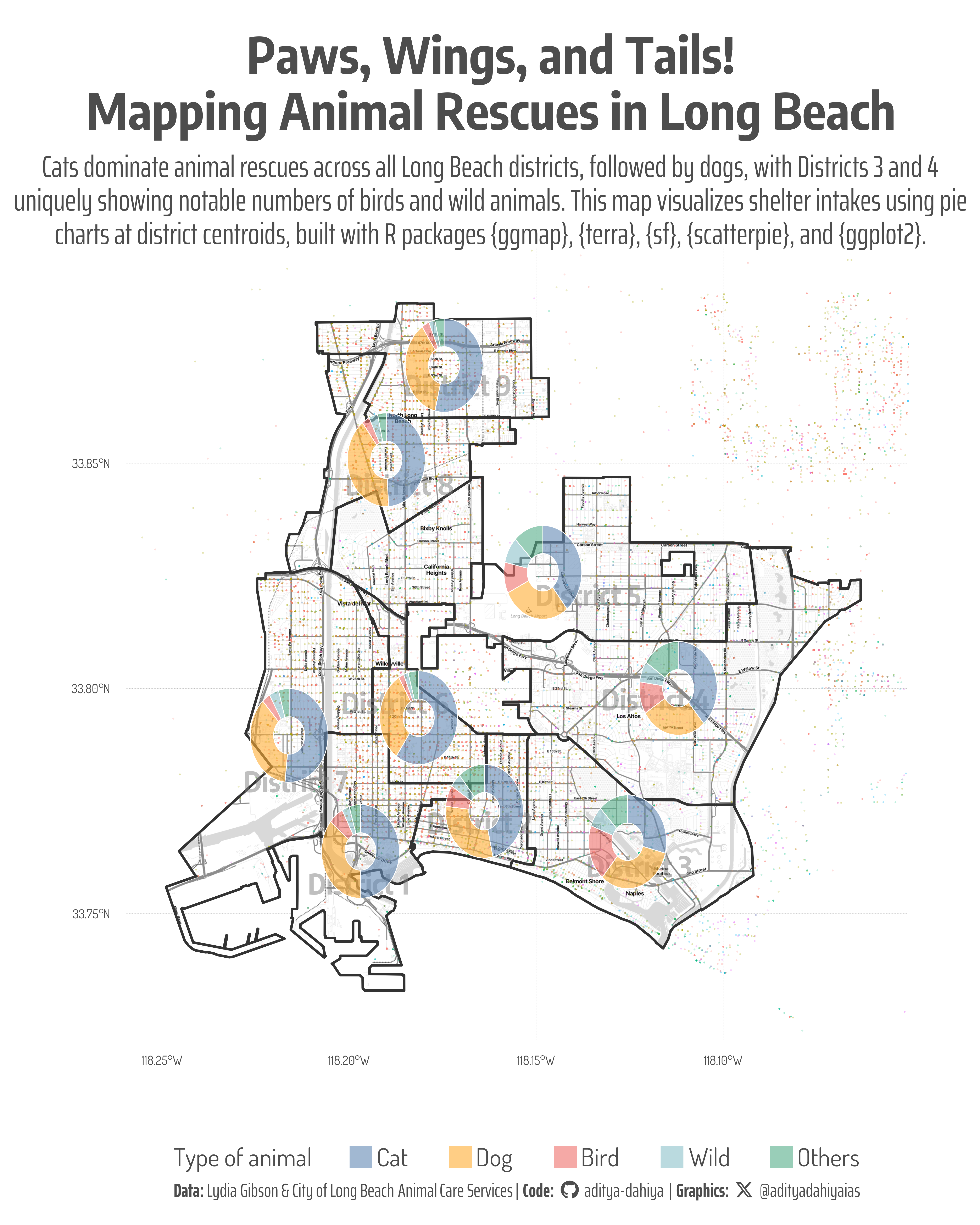
Using the Long Beach Animal Shelter dataset, this graphic maps the locations of rescued animals across the city’s districts, leveraging latitude and longitude data. A base map of Long Beach was sourced from {ggmap} and Stadia Maps, converted to a SpatRaster with {terra}, and cropped to district boundaries for precision. Pie charts, created with {scatterpie} and positioned at district centroids using {sf}, illustrate the distribution of rescued animal types—“Cat,” “Dog,” “Bird,” “Wild,” and “Others”—within each district. The analysis reveals that cats are the most frequently rescued animals across all districts, followed by dogs. Notably, Districts 3 and 4 stand out with significant rescues of birds and wild animals alongside cats and dogs, highlighting distinct regional patterns in animal shelter intakes.

Figure 1: This graphic maps animal rescues across Long Beach districts, with pie charts at district centroids showing the prevalence of cats, dogs, birds, wild animals, and others, revealing cats as the most rescued in all areas and Districts 3 and 4 with notable bird and wild rescues. Created using R with {ggmap} (base map from Stadia Maps), {terra} (raster handling), {sf} (spatial data), {scatterpie} (pie charts), and {ggplot2} (plotting).

How I made this graphic?

Loading required libraries

# Data Import and Wrangling Tools
library(tidyverse)            # All things tidy

# Final plot tools
library(scales)               # Nice Scales for ggplot2
library(fontawesome)          # Icons display in ggplot2
library(ggtext)               # Markdown text support for ggplot2
library(showtext)             # Display fonts in ggplot2
library(colorspace)           # Lighten and Darken colours

# Geocomputation
library(sf)                   # Simple features / maps in R
library(osmdata)              # Getting Open Street Maps data
library(ggmap)                # Get background maps
library(terra)                # Handling rasters in R
library(tidyterra)            # Plotting rasters with ggplot2

longbeach <- readr::read_csv('https://raw.githubusercontent.com/rfordatascience/tidytuesday/main/data/2025/2025-03-04/longbeach.csv')

Visualization Parameters

# Font for titles
font_add_google("Encode Sans Condensed",
  family = "title_font"
) 

# Font for the caption
font_add_google("Saira Extra Condensed",
  family = "caption_font"
) 

# Font for plot text
font_add_google("Dosis",
  family = "body_font"
) 

# Font for background text
font_add_google(
  "Sigmar One",
  family = "back_font"
)

showtext_auto()

mypal <- c("#6388B4", "#FFAE34", "#EF6F6A", "#8CC2CA", "#55AD89")
# cols4all::c4a_gui()

# A base Colour
bg_col <- "white"
seecolor::print_color(bg_col)

# Colour for highlighted text
text_hil <- "grey30"
seecolor::print_color(text_hil)

# Colour for the text
text_col <- "grey30"
seecolor::print_color(text_col)

# Define Base Text Size
bts <- 90 

# Caption stuff for the plot
sysfonts::font_add(
  family = "Font Awesome 6 Brands",
  regular = here::here("docs", "Font Awesome 6 Brands-Regular-400.otf")
)
github <- "&#xf09b"
github_username <- "aditya-dahiya"
xtwitter <- "&#xe61b"
xtwitter_username <- "@adityadahiyaias"
social_caption_1 <- glue::glue("<span style='font-family:\"Font Awesome 6 Brands\";'>{github};</span> <span style='color: {text_hil}'>{github_username}  </span>")
social_caption_2 <- glue::glue("<span style='font-family:\"Font Awesome 6 Brands\";'>{xtwitter};</span> <span style='color: {text_hil}'>{xtwitter_username}</span>")
plot_caption <- paste0(
  "**Data:** Lydia Gibson & City of Long Beach Animal Care Services", 
  " |  **Code:** ", 
  social_caption_1, 
  " |  **Graphics:** ", 
  social_caption_2
  )
rm(github, github_username, xtwitter, 
   xtwitter_username, social_caption_1, 
   social_caption_2)

# Add text to plot-------------------------------------------------
plot_title <- "Paws, Wings, and Tails!\nMapping Animal Rescues in Long Beach"

plot_subtitle <- str_wrap("Cats dominate animal rescues across all Long Beach districts, followed by dogs, with Districts 3 and 4 uniquely showing notable numbers of birds and wild animals. This map visualizes shelter intakes using pie charts at district centroids, built with R packages {ggmap}, {terra}, {sf}, {scatterpie}, and {ggplot2}.", 110)

str_view(plot_subtitle)

Exploratory Data Analysis and Wrangling

Get City of Long Beach district boundaries from official website.

# Try {geodata} to get district boundaries
# longbeach_counties <- geodata::gadm(
#   country = "USA",
#   path = tempdir()
# )

# Trying {tigris} to get districts boundaries  
# library(tigris)
# temp1 <- school_districts(
#   year = 2020, 
#   state = "CA",
#   filter_by = longbeach_bb
#   )

# Try {osmdata} to get district boundaries
longbeach_bb <- osmdata::getbb("Long Beach")
# 
# longbeach_districts <- opq(bbox = longbeach_bb) |> 
#   add_osm_feature(
#     key = "boundary",
#     value = c("administrative")
#   ) |> 
#   osmdata_sf()

library(httr)

# Define the URL
shapefile_url <- "https://data.longbeach.gov/api/explore/v2.1/catalog/datasets/colb-council-districts/exports/shp?lang=en&timezone=Asia%2FKolkata"

# Create a temporary directory
temp_dir <- tempdir()
zip_file <- file.path(tempdir(), "shapefile.zip")

# Download the ZIP file
GET(shapefile_url, write_disk(zip_file, overwrite = TRUE))

# Unzip the downloaded file
unzip(zip_file, exdir = temp_dir)

# Identify the .shp file (assuming it is named 'colb-council-districts.shp')

# Identify the .shp file (assuming it is named 'colb-council-districts.shp')
shp_file <- file.path(temp_dir, "colb-council-districts.shp")

# Read the shapefile into an sf object
council_districts <- st_read(shp_file)

rm(temp_dir, shapefile_url, shp_file, zip_file)

longbeach_districts <- council_districts |>
  mutate(
    district = council_num,
    pop = population,
    area = shape_area,
    geometry = geometry,
    .keep = "none"
  )

# library(summarytools)

# longbeach |> 
#   dfSummary() |> 
#   view()
# 
# longbeach |> names()

# gEt only few types of animals which we can plot
df1 <- longbeach |> 
  mutate(
    animal_type = case_when(
      animal_type == "cat" ~ "Cat",
      animal_type == "dog" ~ "Dog",
      animal_type == "bird" ~ "Bird",
      animal_type == "wild" ~ "Wild",
      .default = "Others"
    ),
    animal_type = fct(
      animal_type,
      levels = c(
        "Cat", "Dog", "Bird", "Wild", "Others"
    ))
  ) |>
  st_as_sf(
    coords = c("longitude", "latitude"),
    crs = "EPSG:4326"
  ) |> 
  select(animal_type, geometry) |> 
  st_join(longbeach_districts)

# Animal Type per district
df2 <- df1 |> 
  st_drop_geometry() |> 
  group_by(district) |> 
  count(animal_type) |> 
  filter(!is.na(district))

# A comparison chart
df2 |> 
  ggplot(
    aes(
      x = district, y = n, fill = animal_type
    )
  ) +
  geom_col(
    position = "fill"
  )

# Convert df2 into a tibble that {scatterpie} can understand
df3 <- df2 |> 
  pivot_wider(
    id_cols = district,
    names_from = animal_type,
    values_from = n
  ) |> 
  mutate(
    total  = Cat + Dog + Bird + Wild + Others
  ) |> 
  
  # Add latitude and longitude from centroids of districts
  left_join(
    council_districts |> 
      mutate(district = council_num) |> 
      select(district, geometry) |> 
      st_centroid() |> 
      mutate(
        longitude = st_coordinates(geometry)[,1],
        latitude = st_coordinates(geometry)[,2]
        ) |> 
      st_drop_geometry()

  )

# Required packages
library(ggmap)
library(terra)
library(ggplot2)
library(tidyterra)

# Get the map from ggmap
# register_stadiamaps("YOUR-API-KEY-HERE")

# Define the bounding box (assuming longbeach_bb is defined elsewhere)
# Example: longbeach_bb <- c(left = -118.25, bottom = 33.75, right = -118.10, top = 33.85)
longbeach_basemap <- get_stadiamap(
  bbox = longbeach_bb,
  zoom = 15,
  maptype = "stamen_toner_lite"
)

# Create a SpatRaster from the {ggmap} base map
spat_raster1 <- rast(longbeach_basemap) |> 
  crop(
    vect(
      council_districts |> 
      st_geometry() |> 
      st_union()
      ),
    mask = TRUE
  )

The Base Plots

Using {scatterpie} package (Yu 2024) for pie-charts.

g <- ggplot(df1) +
  geom_spatraster_rgb(
    data = spat_raster1,
    maxcell = Inf
  ) +
  geom_sf(
    aes(colour = animal_type),
    alpha = 0.2,
    size = 0.4
  ) +
  geom_sf(
    data = longbeach_districts,
    colour = "grey20",
    fill = NA,
    linewidth = 1.4
  ) +
  geom_sf_text(
    data = longbeach_districts,
    aes(label = paste0("District ", district)),
    colour = "grey50",
    size = bts / 2.5,
    nudge_y = -0.005,
    family = "title_font",
    alpha = 0.5,
    fontface = "bold"
  ) +
  scatterpie::geom_scatterpie(
    data = df3,
    aes(
      x = longitude, 
      y = latitude, 
      group = district
    ),
    cols = c(
      "Cat", "Dog", "Bird", "Wild", "Others"
    ),
    colour = bg_col,
    alpha = 0.6,
    donut_radius = 0.4,
    pie_scale = 5,
    linewidth = 0.4
  ) +
  scale_fill_manual(values = mypal) +
  coord_sf(
    xlim = c(-118.25, -118.06),
    ylim = c(33.73, 33.89),
    expand = TRUE,
    default_crs = "EPSG:4326"
  ) +
  guides(
    alpha = "none",
    colour = "none"
  ) +
  labs(
    x = NULL,
    y = NULL,
    colour = NULL,
    subtitle = plot_subtitle,
    title = plot_title,
    caption = plot_caption,
    fill = "Type of animal"
  ) +
  theme_minimal(
    base_family = "body_font",
    base_size = bts
  ) +
  theme(
    
    # Overall Plot
    plot.title.position = "plot",
    text = element_text(
      margin = margin(0,0,0,0, "mm"),
      colour = text_hil,
      hjust = 0.5,
      vjust = 0.5
    ),
    plot.title = element_text(
        margin = margin(10,0,5,0, "mm"),
        colour = text_hil,
        hjust = 0.5,
        size = bts * 2,
        family = "title_font",
        face = "bold",
        lineheight = 0.3
      ),
    plot.subtitle = element_text(
      colour = text_hil,
      size = bts * 1.2,
      hjust = 0.5, 
      vjust = 0.5,
      lineheight = 0.3,
      margin = margin(0,0,0,0, "mm"),
      family = "caption_font"
    ),
    plot.caption = element_textbox(
      halign = 0,
      hjust = 0.5,
      family = "caption_font",
      margin = margin(5,0,5,0, "mm"),
      size = 0.75 * bts
    ),
    plot.margin = margin(5,0,5,0, "mm"),
    panel.background = element_rect(
      fill = "transparent",
      colour = "transparent"
    ),
    plot.background = element_rect(
      fill = "transparent",
      colour = "transparent"
    ),
    
    # Axis and Strips
    axis.text = element_text( 
      size = 0.5 * bts,
      margin = margin(0,0,0,0, "mm")
      ),
    axis.ticks = element_blank(),
    axis.ticks.length = unit(0, "mm"),
    
    # Legend
    legend.position = "bottom",
    legend.text = element_text(
      margin = margin(0,0,0,2, "mm"),
      size = bts
    ),
    legend.key.height = unit(5, "mm"),
    legend.key.width = unit(10, "mm"),
    legend.margin = margin(0,0,0,0, "mm"),
    legend.box.margin = margin(0,0,0,0, "mm"),
    legend.title = element_text(
      lineheight = 0.3,
      margin = margin(0,15,0,0, "mm")
    ),
    
    # Panel Grid
    panel.grid = element_line(
      linetype = 3,
      colour = "grey50",
      linewidth = 0.1
    )
  )

ggsave(
  filename = here::here(
    "data_vizs",
    "tidy_animal_shelter.png"
  ),
  plot = g,
  width = 400,
  height = 500,
  units = "mm",
  bg = bg_col
)

Savings the thumbnail for the webpage

# Saving a thumbnail

library(magick)

# Saving a thumbnail for the webpage
image_read(here::here("data_vizs", 
                      "tidy_animal_shelter.png")) |> 
  image_resize(geometry = "x400") |> 
  image_write(
    here::here(
      "data_vizs", 
      "thumbnails", 
      "tidy_animal_shelter.png"
    )
  )

Session Info

# Data Import and Wrangling Tools
library(tidyverse)            # All things tidy

# Final plot tools
library(scales)               # Nice Scales for ggplot2
library(fontawesome)          # Icons display in ggplot2
library(ggtext)               # Markdown text support for ggplot2
library(showtext)             # Display fonts in ggplot2
library(colorspace)           # Lighten and Darken colours

# Geocomputation
library(sf)                   # Simple features / maps in R
library(osmdata)              # Getting Open Street Maps data
library(ggmap)                # Get background maps
library(terra)                # Handling rasters in R
library(tidyterra)            # Plotting rasters with ggplot2

sessioninfo::session_info()$packages |> 
  as_tibble() |> 
  select(package, 
         version = loadedversion, 
         date, source) |> 
  arrange(package) |> 
  janitor::clean_names(
    case = "title"
  ) |> 
  gt::gt() |> 
  gt::opt_interactive(
    use_search = TRUE
  ) |> 
  gtExtras::gt_theme_espn()

Table 1: R Packages and their versions used in the creation of this page and graphics

References

Yu, Guangchuang. 2024. “Scatterpie: Scatter Pie Plot.” https://CRAN.R-project.org/package=scatterpie.