Five subfamilies, two patterns: mapping Australia’s climate-constrained frog diversity through citizen science.
#TidyTuesday
Maps
{ggforce}
Convex Mark Hull
Author
Aditya Dahiya
Published
August 31, 2025
About the Data
This week’s dataset explores Australian frog biodiversity through the 2023 release of FrogID data, representing the sixth annual publication from this groundbreaking citizen science initiative. FrogID is an innovative mobile app that enables citizen scientists across Australia to record and submit frog calls, which are then expertly identified by museum professionals. Since its launch in 2017, this collaborative effort has generated data that has contributed to over 30 scientific papers examining frog ecology, taxonomy, and conservation. The dataset is particularly significant given that Australia hosts 257 unique native frog species—most found nowhere else on Earth—with nearly one in five species currently threatened with extinction due to climate change, urbanization, disease, and invasive species. The data includes occurrence records with precise geographic coordinates, temporal information, and species identifications validated by experts, offering researchers and data enthusiasts a comprehensive view of Australian frog distributions and calling patterns. This rich dataset, formally documented in ZooKeys by Rowley & Callaghan (2020), provides an invaluable resource for understanding the current state of Australia’s imperiled amphibian fauna and supports ongoing conservation efforts through community-driven scientific discovery.
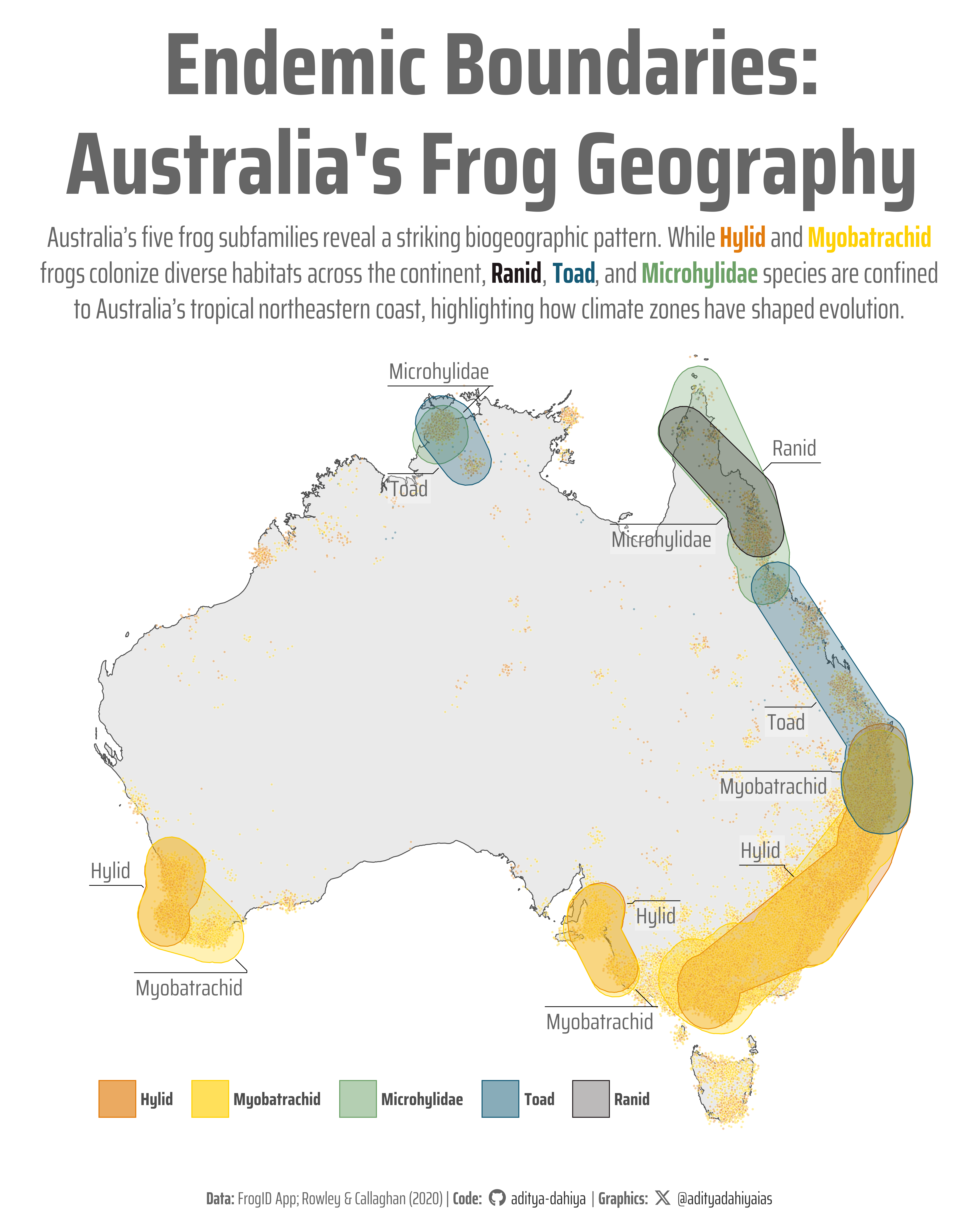
Figure 1: Distribution map based on citizen-contributed frog call recordings shows marked geographic segregation among Australia’s five major amphibian subfamilies. Each dot represents a validated frog call recording from the FrogID citizen science database, with colors indicating the five major Australian frog subfamilies. Shaded regions highlight core distribution areas where each subfamily’s populations are most concentrated. The map demonstrates the stark biogeographic divide between widespread generalist subfamilies (Hylidae and Myobatrachidae) that occur across Australia’s diverse environments, and tropical specialists (Ranidae, Bufonidae, and Microhylidae) restricted to the humid northeastern coastal regions.
How I Made This Graphic
This visualization was created using R with several specialized packages for spatial analysis and advanced plotting techniques. The core data manipulation relied on the tidyverse ecosystem, particularly dplyr for data wrangling and ggplot2 for the base mapping framework. Spatial operations were handled using sf for coordinate transformations and map clipping, while the Australian map boundaries came from rnaturalearth. The key analytical challenge—identifying the 70% most concentrated points for each subfamily—was solved using kernel density estimation through MASS::kde2d() and fields::interp.surface() to calculate density at each point location, then ranking and selecting the highest-density observations. The striking convex hulls that define each subfamily’s core distribution were created using ggforce::geom_mark_hull(), which automatically generates smooth, labeled boundary polygons around point clusters. Additional aesthetic enhancements included the fishualize color palette for subfamily differentiation, ggtext for HTML-formatted text elements with coloured subfamily names, and showtext for custom Google Fonts integration, creating a publication-ready visualization that clearly communicates Australia’s distinct amphibian bio-geographic patterns.
Loading required libraries
Code
pacman::p_load(ggforce)# To plot geom_convex_hull()pacman::p_load(MASS, fields)pacman::p_load( tidyverse, # All things tidy scales, # Nice Scales for ggplot2 fontawesome, # Icons display in ggplot2 ggtext, # Markdown text support for ggplot2 showtext, # Display fonts in ggplot2 colorspace, # Lighten and Darken colours patchwork, # Composing Plots sf # Spatial Operations)# Using RfrogID_data <- readr::read_csv('https://raw.githubusercontent.com/rfordatascience/tidytuesday/main/data/2025/2025-09-02/frogID_data.csv')frog_names <- readr::read_csv('https://raw.githubusercontent.com/rfordatascience/tidytuesday/main/data/2025/2025-09-02/frog_names.csv')
Visualization Parameters
Code
# Font for titlesfont_add_google("Saira",family ="title_font") # Font for the captionfont_add_google("Saira Condensed",family ="body_font") # Font for plot textfont_add_google("Saira Extra Condensed",family ="caption_font") showtext_auto()# A base Colourbg_col <-"white"seecolor::print_color(bg_col)# Colour for highlighted texttext_hil <-"grey40"seecolor::print_color(text_hil)# Colour for the texttext_col <-"grey30"seecolor::print_color(text_col)line_col <-"grey30"# Define Base Text Sizebts <-80# Caption stuff for the plotsysfonts::font_add(family ="Font Awesome 6 Brands",regular = here::here("docs", "Font Awesome 6 Brands-Regular-400.otf"))github <-""github_username <-"aditya-dahiya"xtwitter <-""xtwitter_username <-"@adityadahiyaias"social_caption_1 <- glue::glue("<span style='font-family:\"Font Awesome 6 Brands\";'>{github};</span> <span style='color: {text_hil}'>{github_username} </span>")social_caption_2 <- glue::glue("<span style='font-family:\"Font Awesome 6 Brands\";'>{xtwitter};</span> <span style='color: {text_hil}'>{xtwitter_username}</span>")plot_caption <-paste0("**Data:** FrogID App; Rowley & Callaghan (2020)", " | **Code:** ", social_caption_1, " | **Graphics:** ", social_caption_2 )rm(github, github_username, xtwitter, xtwitter_username, social_caption_1, social_caption_2)# Add text to plot-------------------------------------------------plot_title <-"Endemic Boundaries:\nAustralia's Frog Geography"# Adding Subtitle:# First, get the color palette to match your plotmypal <- paletteer::paletteer_d("fishualize::Balistapus_undulatus")# Create color mapping for subfamiliessubfamily_colors <-setNames( mypal, c("Hylid", "Myobatrachid", "Microhylidae", "Toad", "Ranid"))# Formatted subtitle with ggtext color coding and line breaksplot_subtitle <-paste0("Australia's five frog subfamilies reveal a striking biogeographic pattern. While <span style='color:", subfamily_colors["Hylid"], "'>**Hylid**</span> and <span style='color:", subfamily_colors["Myobatrachid"], "'>**Myobatrachid**</span><br>","frogs colonize diverse habitats across the continent, <span style='color:", subfamily_colors["Ranid"], "'>**Ranid**</span>, <span style='color:", subfamily_colors["Toad"], "'>**Toad**</span>, and <span style='color:", subfamily_colors["Microhylidae"], "'>**Microhylidae**</span> species are confined<br>","to Australia's tropical northeastern coast, highlighting how climate zones have shaped evolution.")str_view(plot_subtitle)# Get a map of Australia to plot# Create bounding box for latitude restrictionclip_polygon <-st_as_sfc(st_bbox(c(xmin =110, ymin =-44, xmax =155, ymax =-8), crs =st_crs(4326) ))# Get Australia map and apply latitude restrictionaus_map <- rnaturalearth::ne_countries(country ="Australia",scale ="large",returnclass ="sf") |> dplyr::select(geometry) |># Clip to latitude bounds before transformingst_intersection(clip_polygon) |># Transform to Australian coordinate systemst_transform(crs =7845)
Exploratory Data Analysis and Wrangling
Code
# Exploring the data to understand it# pacman::p_load(summarytools)# frogID_data |> # dfSummary() |> # view()# # frog_names |> # dfSummary() |> # view()# # pacman::p_unload(summarytools)# Get the data to plot as an SF objectplotdf_points <- frogID_data |># drop uncertain measurementsfilter(coordinateUncertaintyInMeters <100) |># drop out of mainland measurementsfilter( decimalLatitude >-44& decimalLatitude <-8& decimalLongitude >112& decimalLongitude <154 ) |>left_join( frog_names |> dplyr::select(scientificName, subfamily, tribe),relationship ="many-to-many" ) |> janitor::clean_names() |> dplyr::select( event_id, decimal_latitude, decimal_longitude, subfamily, tribe ) |>filter(!is.na(subfamily) &!is.na(tribe)) |>mutate(subfamily =fct( subfamily,levels =c("Hylid", "Myobatrachid", "Microhylidae", "Toad","Ranid" ) ) )# plotdf_points |> # count(subfamily) |> # pull(subfamily)# Function to calculate density-based core points for each subfamilyget_core_points <-function(data, prop =0.5) { data |>group_by(subfamily) |>group_modify(~ {if (nrow(.x) <3) return(.x) # Keep all points if too few for hull# Calculate 2D kernel density coords <-cbind(.x$decimal_longitude, .x$decimal_latitude) kde <- MASS::kde2d(coords[,1], coords[,2], n =50)# Get density at each point location density_at_points <- fields::interp.surface(obj =list(x = kde$x, y = kde$y, z = kde$z),loc = coords )# Select top proportion of points by density n_keep <-ceiling(nrow(.x) * prop) density_rank <-rank(-density_at_points, ties.method ="random") core_mask <- density_rank <= n_keep .x[core_mask, ] }) |>ungroup()}# plotdf_points |> # distinct(subfamily)filter_fams <-c("Hylid", "Myobatrachid")# Create core points dataset (most concentrated 50%)plotdf_core1 <-get_core_points( plotdf_points |>filter(decimal_longitude >140) |>filter(!(subfamily %in% filter_fams & decimal_latitude >-25) ), prop =0.7)plotdf_core2 <-get_core_points( plotdf_points |>filter( decimal_longitude <140& decimal_longitude >120& decimal_latitude >-25&!(subfamily %in% filter_fams) ), prop =0.7)plotdf_core3 <-get_core_points( plotdf_points |>filter( decimal_longitude <140& decimal_longitude >130& decimal_latitude <-25 ), prop =0.7)plotdf_core4 <-get_core_points( plotdf_points |>filter( decimal_longitude <120 ), prop =0.7)
# Saving a thumbnaillibrary(magick)# Saving a thumbnail for the webpageimage_read(here::here("data_vizs", "tidy_australian_frogs.png")) |>image_resize(geometry ="x400") |>image_write( here::here("data_vizs", "thumbnails", "tidy_australian_frogs.png" ) )