A boxplot of capital distribution using {ggplot2}, {paletteer} and {ggtext}
#TidyTuesday
Author
Aditya Dahiya
Published
February 5, 2026
About the Data
This week’s TidyTuesday dataset explores Brazilian companies through the CNPJ (Cadastro Nacional da Pessoa Jurídica) registry, Brazil’s national database of legal entities. The data originates from official records published by the Brazilian Ministry of Finance / Receita Federal on the country’s national open-data portal at dados.gov.br. This large-scale public registry has been cleaned and enriched with lookup tables covering legal nature classifications, owner qualifications, and company size categories, then filtered to focus on firms above a minimum share-capital threshold. The dataset enables analysis of how capital stock concentrates across different legal structures, company sizes, and ownership types in Brazil’s corporate landscape. Special thanks to Marcelo Silva for curating this week’s dataset.
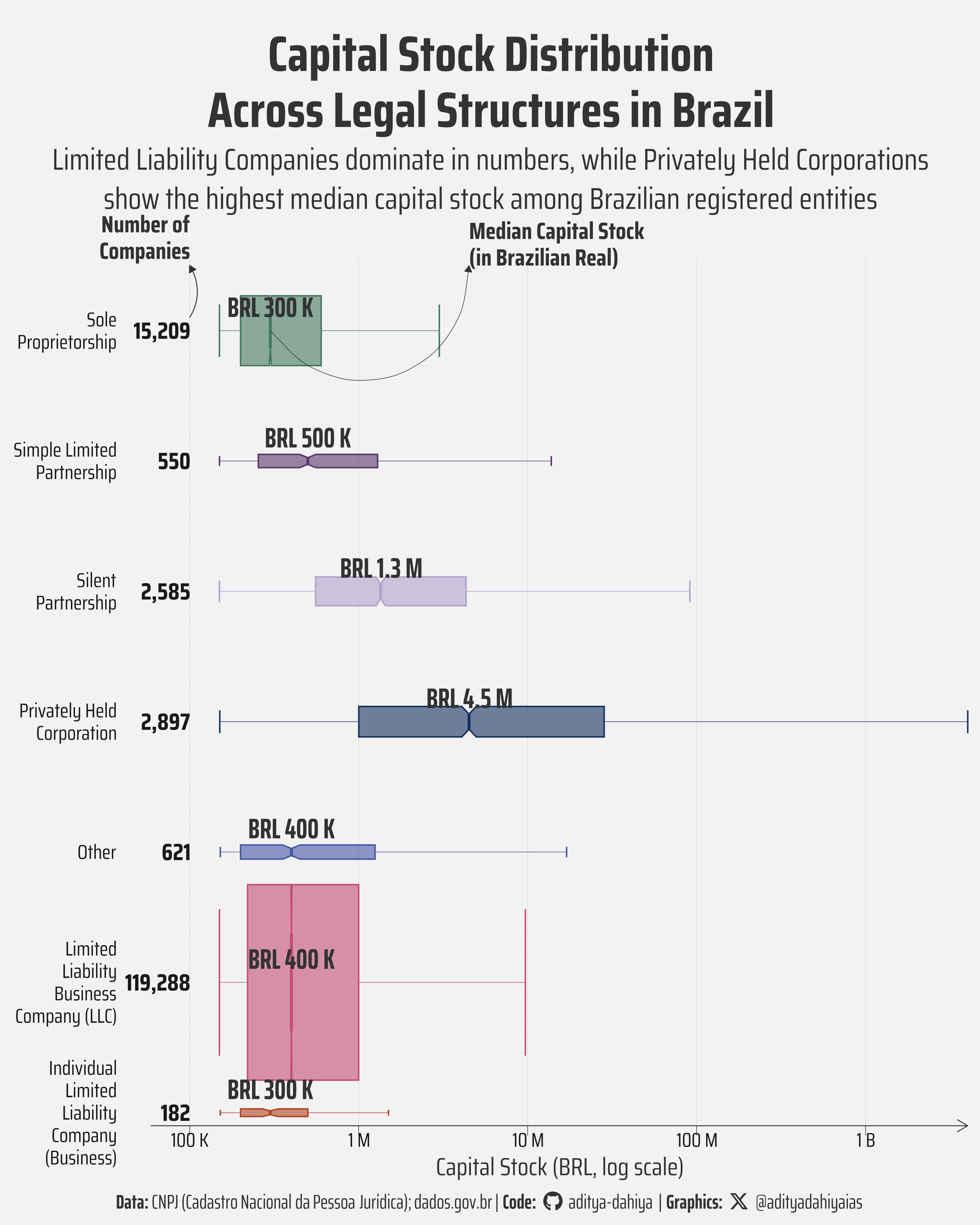
Figure 1: The graph shows the capital stock (in log scale, in Brazilian Real) along the X-axis, and the 7 different legal structures of companies along the Y-axis. Each boxplot’s width corresponds to the total number of companies in that category. The text annotations show number of companies (on left of the boxplots) and the value of median capital stock for each category (i.e. the central line of the boxplot) is labelled.
How I Made This Graphic
Loading required libraries
Code
pacman::p_load( tidyverse, # All things tidy scales, # Nice Scales for ggplot2 fontawesome, # Icons display in ggplot2 ggtext, # Markdown text support for ggplot2 showtext, # Display fonts in ggplot2 colorspace, # Lighten and Darken colours sf, # Spatial Features patchwork, # Composing Plots packcircles, # for hierarchichal packing circles colorspace, # Modify and play with colours, extract dominant colours magick # Playing with images)library(ggdist) # For the raincloud componentslibrary(gghalves) # For half-violin plots (optional alternative)tuesdata <- tidytuesdayR::tt_load(2026, week =4)
Visualization Parameters
Code
# Font for titlesfont_add_google("Saira",family ="title_font")# Font for the captionfont_add_google("Saira Condensed",family ="body_font")# Font for plot textfont_add_google("Saira Extra Condensed",family ="caption_font")showtext_auto()# A base Colourbg_col <-"grey95"seecolor::print_color(bg_col)# Colour for highlighted texttext_hil <-"grey20"seecolor::print_color(text_hil)# Colour for the texttext_col <-"grey10"seecolor::print_color(text_col)# Define Base Text Sizebts <-120# Caption stuff for the plotsysfonts::font_add(family ="Font Awesome 6 Brands",regular = here::here("docs", "Font Awesome 6 Brands-Regular-400.otf"))github <-""github_username <-"aditya-dahiya"xtwitter <-""xtwitter_username <-"@adityadahiyaias"social_caption_1 <- glue::glue("<span style='font-family:\"Font Awesome 6 Brands\";'>{github};</span> <span style='color: {text_hil}'>{github_username} </span>")social_caption_2 <- glue::glue("<span style='font-family:\"Font Awesome 6 Brands\";'>{xtwitter};</span> <span style='color: {text_hil}'>{xtwitter_username}</span>")plot_caption <-paste0("**Data:** CNPJ (Cadastro Nacional da Pessoa Jurídica); dados.gov.br"," | **Code:** ", social_caption_1," | **Graphics:** ", social_caption_2)rm( github, github_username, xtwitter, xtwitter_username, social_caption_1, social_caption_2)plot_title <-"tidy_edible_plants"plot_subtitle <-"ttidy_edible_plants"|>str_wrap(110)
# Saving a thumbnaillibrary(magick)# Saving a thumbnail for the webpageimage_read( here::here("data_vizs","tidy_brazilian_companies.png" ) ) |>image_resize(geometry ="x400") |>image_write( here::here("data_vizs","thumbnails","tidy_brazilian_companies.png" ) )
Session Info
Code
pacman::p_load( tidyverse, # All things tidy scales, # Nice Scales for ggplot2 fontawesome, # Icons display in ggplot2 ggtext, # Markdown text support for ggplot2 showtext, # Display fonts in ggplot2 colorspace # Lighten and Darken colours)sessioninfo::session_info()$packages |>as_tibble() |># The attached column is TRUE for packages that were # explicitly loaded with library() dplyr::filter(attached ==TRUE) |> dplyr::select(package,version = loadedversion, date, source ) |> dplyr::arrange(package) |> janitor::clean_names(case ="title" ) |> gt::gt() |> gt::opt_interactive(use_search =TRUE ) |> gtExtras::gt_theme_espn()
Table 1: R Packages and their versions used in the creation of this page and graphics