The contracting Services Stream for British Library
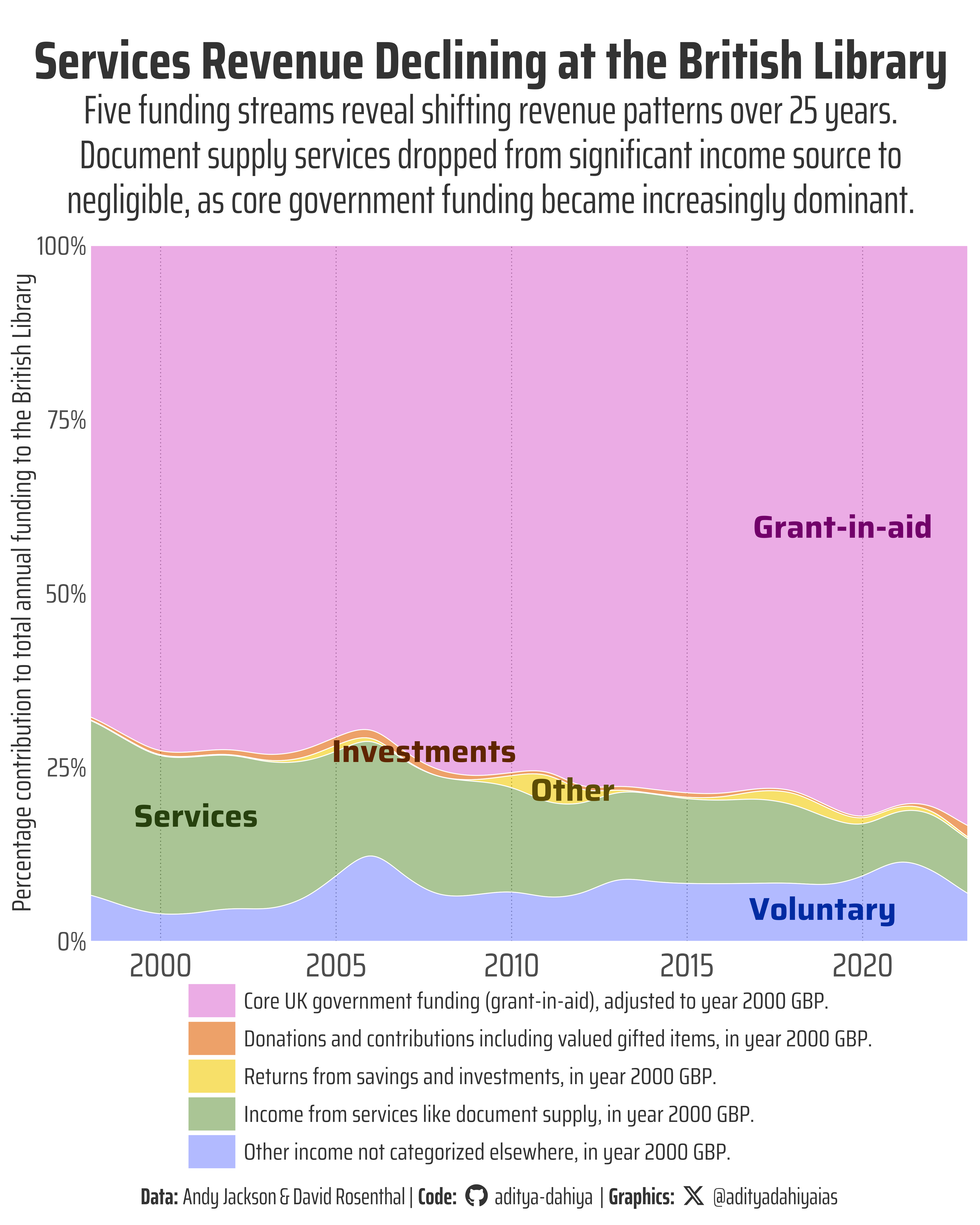
Stream plot showing proportional funding sources from 1999-2024. Services revenue has steadily declined.
#TidyTuesday
Stream Plot
Author
Aditya Dahiya
Published
July 15, 2025
About the Data
This week’s dataset explores the funding patterns of the British Library over the past few decades. Compiled and generously shared by Andy Jackson, the data builds on his earlier post, “Invisible Memory Machines”, and was inspired by David Rosenthal’s 2017 analysis on the decline in inflation-adjusted library income. Andy gathered and cleaned the data with some effort, and later posted updates here and on BlueSky. The dataset, available via this Google Sheet, breaks down British Library funding by source (grant-in-aid, voluntary donations, investments, services, and others) from 1999 onwards, in both nominal and inflation-adjusted terms (using the Bank of England’s inflation calculator). You can load the data in R via the tidytuesdayR package or directly from GitHub. Python and Julia users can explore the dataset using pydytuesday or TidierTuesday.jl. Thanks to Jon Harmon and the Data Science Learning Community for curating this week’s #TidyTuesday dataset.
Figure 1: Stream plot displaying the proportional contribution of five funding sources to British Library’s total annual income from 1999-2024. Data shows grant-in-aid (core government funding), voluntary contributions and donations, investment returns, services revenue, and other income streams. All values adjusted to year 2000 GBP to account for inflation effects over the 25-year period.
How the Graphic Was Created
This stream plot visualization was created using R’s ggplot2 ecosystem with several specialized packages. The core visualization relies on the ggstream package, which provides the geom_stream() function to create proportional stream plots that show how different funding sources contribute to the total over time. You used geom_stream_label() from the same package to add category labels directly onto the stream areas. The data was reshaped using tidyverse functions like pivot_longer() to transform the wide-format funding columns into a long format suitable for the stream plot. Typography was enhanced with showtext to load Google Fonts (Saira family fonts), while ggtext enabled markdown formatting in plot elements like the caption. The color palette was sourced from paletteer and adjusted using colorspace’s darken() function for the text colors. The scales package provided the label_percent() function to format the y-axis as percentages, effectively highlighting the key finding that the Services funding stream (representing income from document supply services) shows a consistent decline in its proportional contribution to the British Library’s total funding over the analyzed period.
Loading required libraries
Code
pacman::p_load( tidyverse, # All things tidy scales, # Nice Scales for ggplot2 fontawesome, # Icons display in ggplot2 ggtext, # Markdown text support for ggplot2 showtext, # Display fonts in ggplot2 colorspace, # Lighten and Darken colours patchwork, # Composing Plots ggstream # Stream Plots with ggplot2)bl_funding <- readr::read_csv('https://raw.githubusercontent.com/rfordatascience/tidytuesday/main/data/2025/2025-07-15/bl_funding.csv')
Visualization Parameters
Code
# Font for titlesfont_add_google("Saira",family ="title_font") # Font for the captionfont_add_google("Saira Condensed",family ="body_font") # Font for plot textfont_add_google("Saira Extra Condensed",family ="caption_font") showtext_auto()# A base Colourbg_col <-"white"seecolor::print_color(bg_col)# Colour for highlighted texttext_hil <-"grey20"seecolor::print_color(text_hil)# Colour for the texttext_col <-"grey20"seecolor::print_color(text_col)line_col <-"grey30"# Define Base Text Sizebts <-120mypal <- paletteer::paletteer_d("fishualize::Balistapus_undulatus")mypal <-c("#DD75D3", "#E16305", "#F2CB05", "#719F4F", "#7E8CFF")# Caption stuff for the plotsysfonts::font_add(family ="Font Awesome 6 Brands",regular = here::here("docs", "Font Awesome 6 Brands-Regular-400.otf"))github <-""github_username <-"aditya-dahiya"xtwitter <-""xtwitter_username <-"@adityadahiyaias"social_caption_1 <- glue::glue("<span style='font-family:\"Font Awesome 6 Brands\";'>{github};</span> <span style='color: {text_hil}'>{github_username} </span>")social_caption_2 <- glue::glue("<span style='font-family:\"Font Awesome 6 Brands\";'>{xtwitter};</span> <span style='color: {text_hil}'>{xtwitter_username}</span>")plot_caption <-paste0("**Data:** Andy Jackson & David Rosenthal", " | **Code:** ", social_caption_1, " | **Graphics:** ", social_caption_2 )rm(github, github_username, xtwitter, xtwitter_username, social_caption_1, social_caption_2)# Add text to plot-------------------------------------------------plot_subtitle <-str_wrap("Five funding streams reveal shifting revenue patterns over 25 years. Document supply services dropped from significant income source to negligible, as core government funding became increasingly dominant.", 75)str_view(plot_subtitle)plot_title <-"Services Revenue Declining at the British Library"
Exploratory Data Analysis and Wrangling
Code
# bl_funding |> # summarytools::dfSummary() |> # summarytools::view()# mutate(# year = as_factor(year)# )# A tibble for labels of the variables I am interested inbl_funding_labels <- tibble::tibble(type =c("gia_y2000_gbp_millions","voluntary_y2000_gbp_millions","investment_y2000_gbp_millions","services_y2000_gbp_millions","other_y2000_gbp_millions" ),short_descrip =c("Grant-in-aid","Voluntary","Investments","Services","Other" ),long_descrip =c("Core UK government funding (grant-in-aid), adjusted to year 2000 GBP.","Donations and contributions including valued gifted items, in year 2000 GBP.","Returns from savings and investments, in year 2000 GBP.","Income from services like document supply, in year 2000 GBP.","Other income not categorized elsewhere, in year 2000 GBP." ))df1 <- bl_funding |>select(year, contains("y2000")) |>select(-contains("total")) |>select(-contains("percentage")) |>pivot_longer(cols =-year,names_to ="type",values_to ="funding" ) |>left_join(bl_funding_labels)
# Saving a thumbnaillibrary(magick)# Saving a thumbnail for the webpageimage_read(here::here("data_vizs", "tidy_british_library_funding.png")) |>image_resize(geometry ="x400") |>image_write( here::here("data_vizs", "thumbnails", "tidy_british_library_funding.png" ) )
Session Info
Code
pacman::p_load( tidyverse, # All things tidy scales, # Nice Scales for ggplot2 fontawesome, # Icons display in ggplot2 ggtext, # Markdown text support for ggplot2 showtext, # Display fonts in ggplot2 colorspace, # Lighten and Darken colours patchwork # Composing Plots)sessioninfo::session_info()$packages |>as_tibble() |> dplyr::select(package, version = loadedversion, date, source) |> dplyr::arrange(package) |> janitor::clean_names(case ="title" ) |> gt::gt() |> gt::opt_interactive(use_search =TRUE ) |> gtExtras::gt_theme_espn()
Table 1: R Packages and their versions used in the creation of this page and graphics