Who Wins British Literary Prizes? A Diversity Analysis
Built with ggplot2, ggstream for flowing visualizations, colorspace for color manipulation, and showtext to integrate Google Fonts
#TidyTuesday
{ggstream}
Author
Aditya Dahiya
Published
October 25, 2025
About the Data
This dataset explores the Selected British Literary Prizes (1990-2022) compiled by the Post45 Data Collective, examining patterns of diversity and representation in British literary prize culture. The data includes comprehensive information on prize winners and shortlisted authors across multiple categories, including gender, sexuality, UK residency status, ethnicity, and educational background with details about degree institutions and fields of study. The dataset enables exploration of questions around which genres see greater representation of women, Black, Asian, and ethnically diverse writers, whether prizes have improved their diversity records over time, and connections between educational credentials and literary recognition. As the authors note, all information is publicly available, though they emphasize the data is intended for studying broad patterns rather than making definitive claims about individuals. Additional metadata discussion provides deeper context on the ethnicity, gender, sexuality, and educational classification variables. The dataset was curated by Jen Richmond for TidyTuesday, following a suggestion by @gkaramanis, and is accessible through R, Python, and Julia workflows.
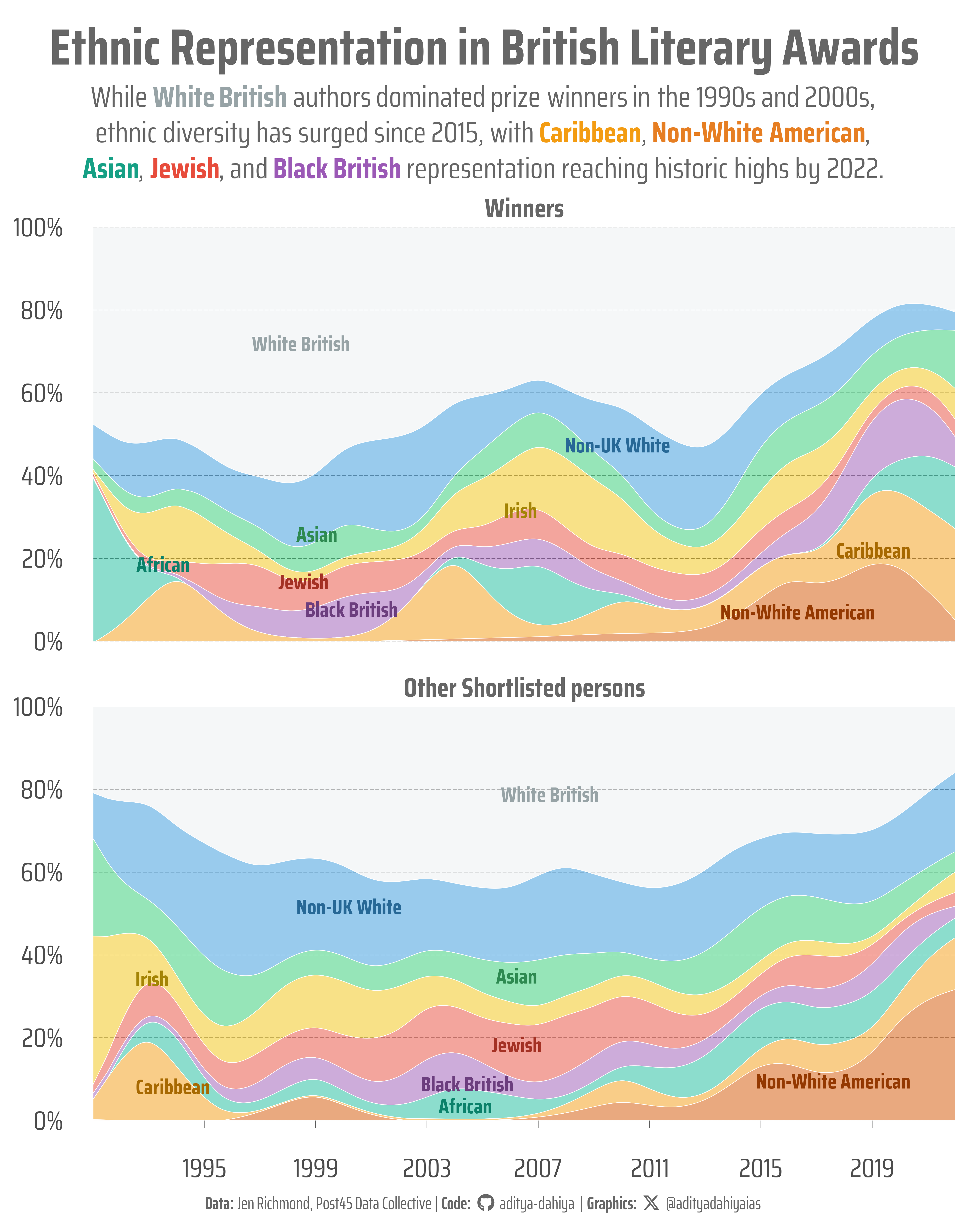
Figure 1: Proportional streamgraph showing ethnic diversity trends in British literary prizes across three decades. Each colored stream represents an ethnic group’s share of prize recipients by year, with the top panel showing winners and bottom panel showing other shortlisted persons. The x-axis spans 1990-2022, while the y-axis represents percentage composition (0-100%). Notable findings include decreasing White British dominance and increasing representation of Caribbean, Non-White American, Asian, and other ethnic minority authors, especially post-2015.
How I Made This Graphic
This visualization was created using R and the tidyverse ecosystem for data manipulation and plotting. The graphic employs ggstream::geom_stream() to create proportional streamgraphs that elegantly show the changing ethnic composition of British literary prize winners and shortlisted authors over time, with ggstream::geom_stream_label() adding labels directly onto the flowing streams. Color palettes were sourced from paletteer using the “flat_dark” theme from ggthemr, with colors further enhanced using colorspace::darken() for better label contrast. Typography was handled through showtext to incorporate Google Fonts (Saira family), while ggtext enabled markdown formatting in plot text elements. The scales package provided clean percentage formatting for the y-axis, and patchwork was loaded for potential plot composition. Faceting with custom labels separated winners from other shortlisted individuals, creating a compelling visual narrative of diversity trends in British literary prizes from 1990 to 2022.
Loading required libraries
Code
pacman::p_load( tidyverse, # All things tidy scales, # Nice Scales for ggplot2 fontawesome, # Icons display in ggplot2 ggtext, # Markdown text support for ggplot2 showtext, # Display fonts in ggplot2 colorspace, # Lighten and Darken colours patchwork # Composing Plots)prizes <- readr::read_csv('https://raw.githubusercontent.com/rfordatascience/tidytuesday/main/data/2025/2025-10-28/prizes.csv')
Visualization Parameters
Code
# Font for titlesfont_add_google("Saira",family ="title_font")# Font for the captionfont_add_google("Saira Condensed",family ="body_font")# Font for plot textfont_add_google("Saira Extra Condensed",family ="caption_font")showtext_auto()# A base Colourbg_col <-"white"seecolor::print_color(bg_col)# Colour for highlighted texttext_hil <-"grey40"seecolor::print_color(text_hil)# Colour for the texttext_col <-"grey30"seecolor::print_color(text_col)line_col <-"grey30"# Define Base Text Sizebts <-80# Caption stuff for the plotsysfonts::font_add(family ="Font Awesome 6 Brands",regular = here::here("docs", "Font Awesome 6 Brands-Regular-400.otf"))github <-""github_username <-"aditya-dahiya"xtwitter <-""xtwitter_username <-"@adityadahiyaias"social_caption_1 <- glue::glue("<span style='font-family:\"Font Awesome 6 Brands\";'>{github};</span> <span style='color: {text_hil}'>{github_username} </span>")social_caption_2 <- glue::glue("<span style='font-family:\"Font Awesome 6 Brands\";'>{xtwitter};</span> <span style='color: {text_hil}'>{xtwitter_username}</span>")plot_caption <-paste0("**Data:** Jen Richmond, Post45 Data Collective"," | **Code:** ", social_caption_1," | **Graphics:** ", social_caption_2)rm( github, github_username, xtwitter, xtwitter_username, social_caption_1, social_caption_2)# Add text to plot-------------------------------------------------plot_title <-"Ethnic Representation in British Literary Awards"plot_subtitle <- plot_subtitle <-"While <span style='color:#97A3A6;'>**White British**</span> authors dominated prize winners in the 1990s and 2000s,<br>ethnic diversity has surged since 2015, with <span style='color:#F39C12;'>**Caribbean**</span>, <span style='color:#E67E22;'>**Non-White American**</span>,<br><span style='color:#16A085;'>**Asian**</span>, <span style='color:#E74C3C;'>**Jewish**</span>, and <span style='color:#9B59B6;'>**Black British**</span> representation reaching historic highs by 2022."
# Saving a thumbnaillibrary(magick)# Saving a thumbnail for the webpageimage_read(here::here("data_vizs","tidy_british_literary_prizes.png")) |>image_resize(geometry ="x400") |>image_write( here::here("data_vizs","thumbnails","tidy_british_literary_prizes.png" ) )
Session Info
Code
sessioninfo::session_info()$packages |>as_tibble() |># The attached column is TRUE for packages that were # explicitly loaded with library() dplyr::filter(attached ==TRUE) |> dplyr::select(package,version = loadedversion, date, source ) |> dplyr::arrange(package) |> janitor::clean_names(case ="title" ) |> gt::gt() |> gt::opt_interactive(use_search =TRUE ) |> gtExtras::gt_theme_espn()
Table 1: R Packages and their versions used in the creation of this page and graphics