Patterns in Purged Data: Most Common Tags

Visualizing common themes in Data: Using {ggplot2} and {packcircles} to Uncover Patterns

About the Data

The CDC Datasets for this week’s TidyTuesday focus on publicly available health data. Efforts have been made to archive these datasets on archive.org to preserve critical health data. The dataset contains metadata on these archived resources, including bureau and program codes sourced from the OMB Circular A-11 and the Federal Program Inventory. Key variables include dataset URLs, contact information, program categories, access levels, and update frequency. The data can be accessed via the tidytuesdayR package or directly from GitHub.

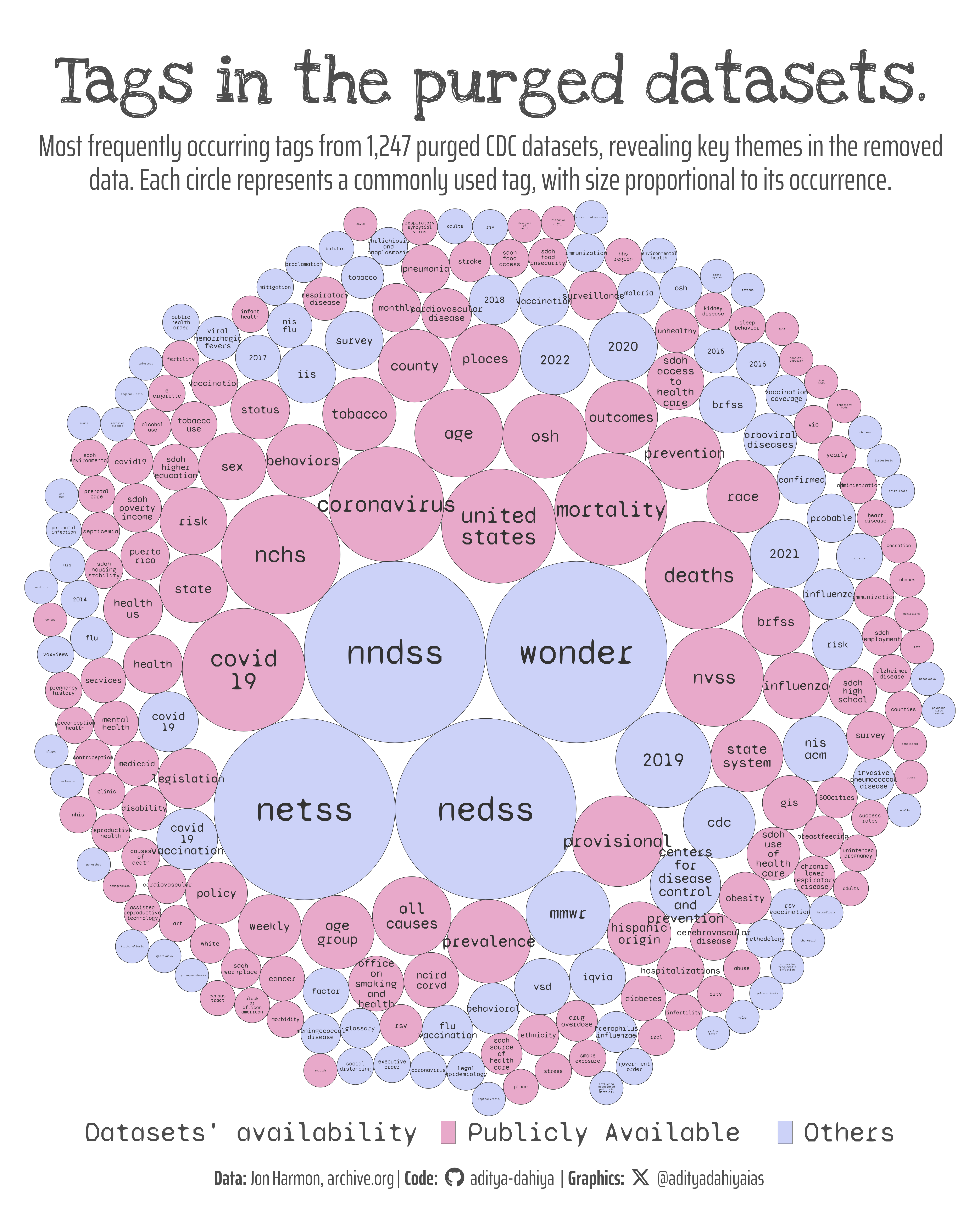
Figure 1: A packcircles visualization of the most frequent tags from 1,247 purged CDC datasets, sized by occurrence and colored by public access status. Created using R with {ggplot2} for plotting and {packcircles} for circle packing.

How I made this graphic?

Loading required libraries

# Data Import and Wrangling Tools
library(tidyverse)            # All things tidy

# Final plot tools
library(scales)               # Nice Scales for ggplot2
library(fontawesome)          # Icons display in ggplot2
library(ggtext)               # Markdown text support for ggplot2
library(showtext)             # Display fonts in ggplot2
library(colorspace)           # Lighten and Darken colours
library(packcircles)          # Pack-Circle Algorithm
# Option 2: Read directly from GitHub

cdc_datasets <- readr::read_csv('https://raw.githubusercontent.com/rfordatascience/tidytuesday/main/data/2025/2025-02-11/cdc_datasets.csv')
fpi_codes <- readr::read_csv('https://raw.githubusercontent.com/rfordatascience/tidytuesday/main/data/2025/2025-02-11/fpi_codes.csv')
omb_codes <- readr::read_csv('https://raw.githubusercontent.com/rfordatascience/tidytuesday/main/data/2025/2025-02-11/omb_codes.csv')

Visualization Parameters

# Font for titles
font_add_google("Love Ya Like A Sister",
  family = "title_font"
) 

# Font for the caption
font_add_google("Saira Extra Condensed",
  family = "caption_font"
) 

# Font for plot text
font_add_google("Syne Mono",
  family = "body_font"
) 

font_add_google(
  "Syne Mono",
  family = "circle_font"
)
showtext_auto()

# A base Colour
bg_col <- "white"
seecolor::print_color(bg_col)

# Colour for highlighted text
text_hil <- "grey30"
seecolor::print_color(text_hil)

# Colour for the text
text_col <- "grey20"
seecolor::print_color(text_col)

# Define Base Text Size
bts <- 90 

# Caption stuff for the plot
sysfonts::font_add(
  family = "Font Awesome 6 Brands",
  regular = here::here("docs", "Font Awesome 6 Brands-Regular-400.otf")
)
github <- "&#xf09b"
github_username <- "aditya-dahiya"
xtwitter <- "&#xe61b"
xtwitter_username <- "@adityadahiyaias"
social_caption_1 <- glue::glue("<span style='font-family:\"Font Awesome 6 Brands\";'>{github};</span> <span style='color: {text_hil}'>{github_username}  </span>")
social_caption_2 <- glue::glue("<span style='font-family:\"Font Awesome 6 Brands\";'>{xtwitter};</span> <span style='color: {text_hil}'>{xtwitter_username}</span>")
plot_caption <- paste0(
  "**Data:** Jon Harmon, archive.org", 
  " |  **Code:** ", 
  social_caption_1, 
  " |  **Graphics:** ", 
  social_caption_2
  )
rm(github, github_username, xtwitter, 
   xtwitter_username, social_caption_1, 
   social_caption_2)

# Add text to plot-------------------------------------------------
plot_title <- "Patterns in Purged Data: Most Common Tags"

plot_subtitle <- "Most frequently occurring tags from 1,247 purged CDC datasets, revealing key themes in the removed data. Each circle represents a commonly used tag, with size proportional to its occurrence."

Exploratory Data Analysis and Wrangling

# library(summarytools)
# cdc_datasets |> 
#   dfSummary() |> 
#   view()
# 
# fpi_codes |>
#   dfSummary() |>
#   view()

# omb_codes |> 
#   dfSummary() |> 
#   view()

df1 <- cdc_datasets |> 
  # left_join(
  #   fpi_codes, by = join_by(program_code == program_code_pod_format)
  # ) |> 
  mutate(
    public = case_when(
      public_access_level == "public" ~ "Publicly Available",
      is.na(public_access_level) ~ "Others",
      .default = "Others"
    ),
    public = fct(public,
                 levels = c(
                   "Publicly Available",
                   "Others"
                 ))
  ) |> 
  rename(fill_var = public) |> 
  separate_longer_delim(cols = tags, delim = ", ") |> 
  count(fill_var, tags, sort = T) |> 
  filter(n >= 10) |> 
  filter(!str_detect(tags, "does not have")) |> 
  mutate(tags = str_replace_all(tags, " ", "\n")) |> 
  mutate(tags = str_replace_all(tags, "-", "\n"))

Create {packcircles} layout

library(packcircles)

# Create the layout using circleProgressiveLayout()
# This function returns a dataframe with a row for each bubble.
# It includes the center coordinates (x and y) and the radius, which is proportional to the value.
packing1 <- circleProgressiveLayout(
  df1$n,
  sizetype = "area"
)

# A tibble of centres of the circles and our cleaned data
plotdf <- bind_cols(
  df1,
  packing1
) |> 
  mutate(id = row_number())

# A tibble of the points on the circumference of the circles
plotdf_circles <- circleLayoutVertices(
  packing1,
  npoints = 100
  ) |> 
  as_tibble() |>
  mutate(id = as.numeric(id)) |> 
  
  # Adding the other variables
  left_join(
    plotdf |> select(-x, -y), by = join_by(id == id)
  )

# Check if everything worked.
# visdat::vis_miss(plotdf_circles)

The Base Plot

g <- ggplot() +
  
  # Drawing the circles
  geom_polygon(
    data = plotdf_circles,
    mapping = aes(
      x, 
      y, 
      group = id, 
      fill = fill_var
    ),
    colour = text_col,
    linewidth = 0.2,
    alpha = 0.9
  ) +
  
  # Add text at center of each bubble
  geom_text(
    data = plotdf,
    mapping = aes(
      x = x, y = y, 
      label = tags, 
      size = n
    ),
    colour = text_col,
    family = "body_font",
    lineheight = 0.25
  ) +
  
  # Fill colours
  paletteer::scale_fill_paletteer_d("wesanderson::GrandBudapest2") +
  scale_size_continuous(
    range = c(bts / 25, bts / 2)
  ) +
  scale_x_continuous(expand = expansion(0)) +
  scale_y_continuous(expand = expansion(0)) +
  labs(
    title = plot_title,
    subtitle = str_wrap(plot_subtitle, 100),
    caption = plot_caption
  ) +
  guides(
    size = "none",
    fill = guide_legend(
      title = "Datasets' availability",
      override.aes = list(
        shape = 20
      )
    )
  ) +
  coord_equal() +
  theme_void(
    base_size = bts,
    base_family = "caption_font"
  ) +
  theme(
    legend.position = "bottom",
    plot.caption = element_textbox(
      colour = text_hil,
      family = "caption_font",
      hjust = 0.5,
      margin = margin(10,0,0,0, "mm")
    ),
    plot.title = element_text(
      hjust = 0.5,
      size = 2.7 * bts,
      colour = text_hil,
      margin = margin(10,0,0,0, "mm"),
      family = "title_font"
    ),
    plot.subtitle = element_text(
      colour = text_hil,
      size = 1.2 * bts,
      hjust = 0.5, 
      lineheight = 0.3,
      margin = margin(5,0,2,0, "mm"),
      family = "caption_font"
    ),
    legend.title = element_text(
      colour = text_hil,
      margin = margin(0,10,0,0, "mm"),
      hjust = 0.5,
      size = 1.1 * bts,
      family = "body_font"
    ),
    legend.text = element_text(
      colour = text_hil,
      margin = margin(0,0,0,5, "mm"),
      size = 1.1 * bts,
      family = "body_font"
    ),
    plot.margin = margin(10,10,10,10, "mm")
  )


ggsave(
  filename = here::here(
    "data_vizs",
    "tidy_cdc_datasets.png"
  ),
  plot = g,
  width = 400,
  height = 500,
  units = "mm",
  bg = bg_col
)

Savings the thumbnail for the webpage

# Saving a thumbnail

library(magick)

# Saving a thumbnail for the webpage
image_read(here::here("data_vizs", 
                      "tidy_cdc_datasets.png")) |> 
  image_resize(geometry = "x400") |> 
  image_write(
    here::here(
      "data_vizs", 
      "thumbnails", 
      "tidy_cdc_datasets.png"
    )
  )

Session Info

# Data Import and Wrangling Tools
library(tidyverse)            # All things tidy

# Final plot tools
library(scales)               # Nice Scales for ggplot2
library(fontawesome)          # Icons display in ggplot2
library(ggtext)               # Markdown text support for ggplot2
library(showtext)             # Display fonts in ggplot2
library(colorspace)           # Lighten and Darken colours
library(packcircles)          # Pack-Circle Algorithm
sessioninfo::session_info()$packages |> 
  as_tibble() |> 
  select(package, 
         version = loadedversion, 
         date, source) |> 
  arrange(package) |> 
  janitor::clean_names(
    case = "title"
  ) |> 
  gt::gt() |> 
  gt::opt_interactive(
    use_search = TRUE
  ) |> 
  gtExtras::gt_theme_espn()

Table 1: R Packages and their versions used in the creation of this page and graphics