Tracking Cranes at Lake Hornborgasjön

How observation patterns reveal seasonal stopover behavior (1994-2024)

#TidyTuesday
Author

Aditya Dahiya

Published

October 5, 2025

About the Data

This dataset documents crane observations at Lake Hornborgasjön in Västergötland, Sweden, spanning over 30 years of migration patterns. The data comes from dedicated crane counters at the Hornborgasjön field station, who have systematically recorded crane populations during spring and fall migrations. The timing of peak crane presence varies depending on weather conditions—particularly the arrival of spring and favorable southerly winds that support crane flight. The dataset includes daily observation counts, dates, and important contextual notes from counting officials, such as records of bad weather, canceled counts, seasonal milestones (first and last counts), record observations, severe interference, and uncertain counts. Weather disruptions are specifically flagged when original comments mention conditions like fog, rain, snow, thunder, or other adverse weather. This rich historical record enables analysis of population trends, seasonal patterns, and the relationship between crane migration and weather conditions. More information about crane statistics can be found on the Hornborgasjön website.

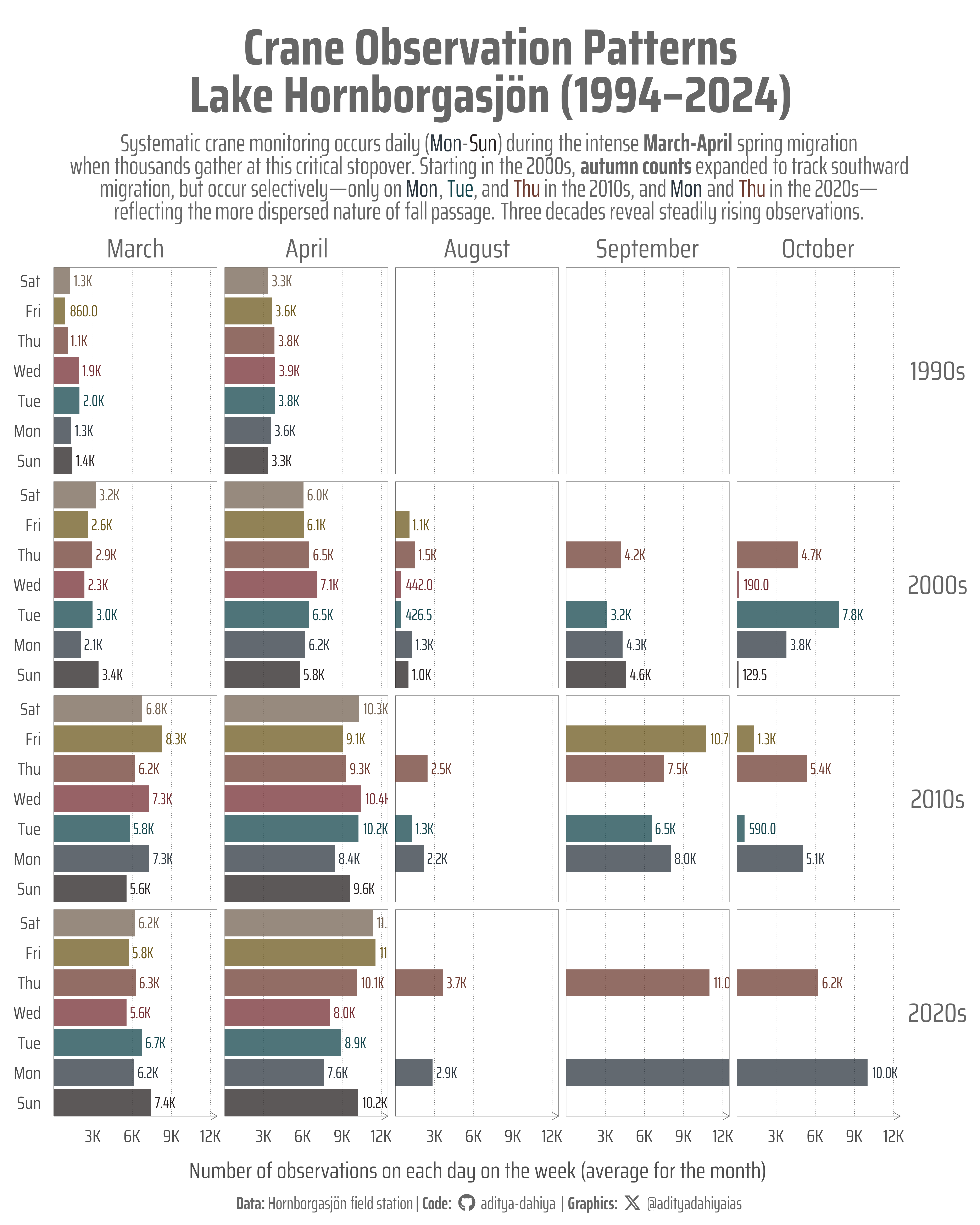
Figure 1: Visualization shows mean crane observations by weekday (y-axis), faceted by month (columns) and decade (rows). Bar length represents average observation count for each day-month-decade combination, with numeric labels showing exact values. Spring months (March-April) display comprehensive daily monitoring across all seven weekdays, while autumn months (August-October) show strategic sampling on selected days only. Growing bar lengths across decades indicate increasing observation frequencies. Colors distinguish weekdays using the Ghibli PonyoDark palette. Data: Hornborgasjön field station crane counts (1994-2024). Missing bars indicate no observations recorded for that weekday-month combination.

How I Made This Graphic

Loading required libraries

Code
pacman::p_load(
  tidyverse, # All things tidy

  scales, # Nice Scales for ggplot2
  fontawesome, # Icons display in ggplot2
  ggtext, # Markdown text support for ggplot2
  showtext, # Display fonts in ggplot2
  colorspace, # Lighten and Darken colours

  patchwork  # Composing Plots
)

cranes <- readr::read_csv('https://raw.githubusercontent.com/rfordatascience/tidytuesday/main/data/2025/2025-09-30/cranes.csv')

Visualization Parameters

Code
# Font for titles
font_add_google("Saira",
  family = "title_font"
)

# Font for the caption
font_add_google("Saira Condensed",
  family = "body_font"
)

# Font for plot text
font_add_google("Saira Extra Condensed",
  family = "caption_font"
)

showtext_auto()

# A base Colour
bg_col <- "white"
seecolor::print_color(bg_col)

# Colour for highlighted text
text_hil <- "grey40"
seecolor::print_color(text_hil)

# Colour for the text
text_col <- "grey30"
seecolor::print_color(text_col)

line_col <- "grey30"

# Define Base Text Size
bts <- 80

# Get the actual colors from chosen palette
day_colors <- paletteer::paletteer_d("ghibli::PonyoDark", n = 7)
names(day_colors) <- c("Sun", "Mon", "Tue", "Wed", "Thu", "Fri", "Sat")

# Caption stuff for the plot
sysfonts::font_add(
  family = "Font Awesome 6 Brands",
  regular = here::here("docs", "Font Awesome 6 Brands-Regular-400.otf")
)
github <- "&#xf09b"
github_username <- "aditya-dahiya"
xtwitter <- "&#xe61b"
xtwitter_username <- "@adityadahiyaias"
social_caption_1 <- glue::glue("<span style='font-family:\"Font Awesome 6 Brands\";'>{github};</span> <span style='color: {text_hil}'>{github_username}  </span>")
social_caption_2 <- glue::glue("<span style='font-family:\"Font Awesome 6 Brands\";'>{xtwitter};</span> <span style='color: {text_hil}'>{xtwitter_username}</span>")
plot_caption <- paste0(
  "**Data:**  Hornborgasjön field station",
  " |  **Code:** ",
  social_caption_1,
  " |  **Graphics:** ",
  social_caption_2
)
rm(
  github, github_username, xtwitter,
  xtwitter_username, social_caption_1,
  social_caption_2
)

# Add text to plot-------------------------------------------------
plot_title <- "Crane Observation Patterns\nLake Hornborgasjön (1994–2024)"

plot_subtitle <- glue::glue(
  "Systematic crane monitoring occurs daily (<span style='color:{day_colors['Mon']}'>Mon</span>-<span style='color:{day_colors['Sun']}'>Sun</span>) during the intense <b>March-April</b> spring migration<br>",
  "when thousands gather at this critical stopover. Starting in the 2000s, <b>autumn counts</b> expanded to track southward<br>",
  "migration, but occur selectively—only on <span style='color:{day_colors['Mon']}'>Mon</span>, <span style='color:{day_colors['Tue']}'>Tue</span>, and <span style='color:{day_colors['Thu']}'>Thu</span> in the 2010s, and <span style='color:{day_colors['Mon']}'>Mon</span> and <span style='color:{day_colors['Thu']}'>Thu</span> in the 2020s—<br>",
  "reflecting the more dispersed nature of fall passage. Three decades reveal steadily rising observations."
)

str_view(plot_subtitle)

Exploratory Data Analysis and Wrangling

Code
# pacman::p_load(summarytools)
# 
# cranes |> 
#   dfSummary() |> 
#   view()
# 
# pacman::p_unload(summarytools)

df1 <- cranes |> 
  mutate(
    year = year(date),
    decade = (year(date) %/% 10) * 10,
    decade_label = paste0(decade, "s"),       # Decade with 's' suffix (1990s, 2000s, etc.)
    month = month(date, label = TRUE, abbr = FALSE),
    day_of_week = wday(date, label = TRUE),
    day = day(date),
    day_of_year = yday(date)
  ) |> 
  filter(!is.na(observations))

df1 |> 
  ggplot(aes(date, observations)) +
  geom_line()

df1 |> 
  group_by(month) |> 
  summarise(
    observations = mean(observations, na.rm = TRUE)
  ) |> 
  ggplot(aes(month, observations)) +
  geom_col()


df1 |> 
  group_by(month, day_of_week) |> 
  summarise(
    observations = mean(observations, na.rm = TRUE)
  ) |> 
  ggplot(aes(day_of_week, observations)) +
  geom_col() +
  facet_wrap(~month)

df1 |> 
  group_by(month, day_of_week) |> 
  summarise(
    observations = mean(observations, na.rm = TRUE)
  ) |> 
  ggplot(aes(day_of_week, observations)) +
  geom_col() +
  facet_wrap(~month)

df1 |> 
  group_by(month, year, day_of_week) |> 
  summarise(
    observations = mean(observations, na.rm = TRUE)
  ) |> 
  ggplot(
    aes(
      x = day_of_week, 
      y = observations, 
      group = as_factor(year),
      colour = as_factor(year)
    )
  ) +
  geom_line() +
  facet_wrap(~month)

The Plot

Code
g <- df1 |> 
  group_by(decade_label, day_of_week, month) |> 
  summarise(
    observations = mean(observations, na.rm = TRUE)
  ) |> 
  ggplot(
    aes(
      y = day_of_week, 
      x = observations,
      fill = day_of_week
    )
  ) +
  geom_col(
    alpha = 0.75
  ) +
  geom_text(
    mapping = aes(
      label = number(
        observations, 
        scale_cut = cut_short_scale(),
        accuracy = 0.1
      ),
      colour = day_of_week
    ),
    hjust = -0.2,
    size = bts / 4,
    family = "caption_font"
  ) +
  facet_grid(decade_label ~ month) +
  scale_fill_manual(
    values = day_colors
  ) +
  scale_colour_manual(
    values = day_colors
  ) +
  scale_x_continuous(
    labels = scales::label_number(scale_cut = cut_short_scale()),
    expand = expansion(0),
    breaks = seq(3, 12, 3) * 1e3
  ) +
  scale_y_discrete(
    expand = expansion(0)
  ) +
  labs(
    title = plot_title,
    subtitle = plot_subtitle,
    caption = plot_caption,
    y = NULL,
    x = "Number of observations on each day on the week (average for the month)",
    colour = NULL,
    fill = NULL
  ) +
  theme_minimal(
    base_family = "body_font",
    base_size = bts
  ) +
  theme(
    legend.position = "none",
    
    # Overall
    text = element_text(
      margin = margin(0, 0, 0, 0, "mm"),
      colour = text_col,
      lineheight = 0.3
    ),
    
    # Axes
    axis.text = element_text(
      margin = margin(2,2,2,2, "mm")
    ),
    axis.ticks.y = element_blank(),
    axis.ticks.x = element_blank(),
    axis.ticks.length = unit(0, "mm"),
    axis.line.y = element_line(
      linewidth = 0.3,
      colour = line_col
    ),
    axis.line.x = element_line(
      arrow = arrow(length = unit(3, "mm")),
      linewidth = 0.3,
      colour = text_hil
    ),
    axis.title.y = element_text(
      margin = margin(0,3,0,0, "mm"),
      colour = text_hil,
      size = bts
    ),
    panel.grid = element_blank(),
    panel.grid.major.x = element_line(
      linetype = 3,
      linewidth = 0.3,
      colour = text_hil
    ),
    panel.background = element_rect(
      fill = NA,
      colour = text_hil,
      linewidth = 0.3
    ),
    
    # Strip Labels
    strip.text.x = element_text(
      colour = text_hil, 
      size = bts * 1.2,
      margin = margin(0,0,3,0, "mm")
    ),
    strip.text.y = element_text(
      colour = text_hil, 
      size = bts * 1.2,
      margin = margin(0,0,0,3, "mm"),
      angle = 0
    ),
    panel.spacing.x = unit(3, "mm"),
    panel.spacing.y = unit(3, "mm"),
    
    # Labels and Strip Text
    plot.title = element_text(
      margin = margin(5, 0, 5, 0, "mm"),
      hjust = 0.5,
      vjust = 0.5,
      colour = text_hil,
      size = 2.3 * bts,
      family = "body_font",
      face = "bold",
      lineheight = 0.25
    ),
    plot.subtitle = element_textbox(
      margin = margin(2, 0, 5, 0, "mm"),
      vjust = 0.5,
      colour = text_hil,
      size = 1.1 * bts,
      hjust = 0.5,
      halign = 0.5,
      family = "caption_font",
      lineheight = 0.3
    ),
    plot.caption = element_markdown(
      family = "caption_font",
      hjust = 0.5,
      margin = margin(5,0,0,0, "mm"),
      colour = text_hil
    ),
    plot.caption.position = "plot",
    plot.title.position = "plot",
    plot.margin = margin(5, 5, 5, 5, "mm")
  )

ggsave(
  filename = here::here(
    "data_vizs",
    "tidy_crane_observations.png"
  ),
  plot = g,
  width = 400,
  height = 500,
  units = "mm",
  bg = bg_col
)

Savings the thumbnail for the webpage

Code
# Saving a thumbnail

library(magick)

# Saving a thumbnail for the webpage
image_read(here::here(
  "data_vizs",
  "tidy_crane_observations.png"
)) |>
  image_resize(geometry = "x400") |>
  image_write(
    here::here(
      "data_vizs",
      "thumbnails",
      "tidy_crane_observations.png"
    )
  )

Session Info

Code
sessioninfo::session_info()$packages |>
  as_tibble() |>
  dplyr::select(package,
    version = loadedversion,
    date, source
  ) |>
  dplyr::arrange(package) |>
  janitor::clean_names(
    case = "title"
  ) |>
  gt::gt() |>
  gt::opt_interactive(
    use_search = TRUE
  ) |>
  gtExtras::gt_theme_espn()
Table 1: R Packages and their versions used in the creation of this page and graphics

Links