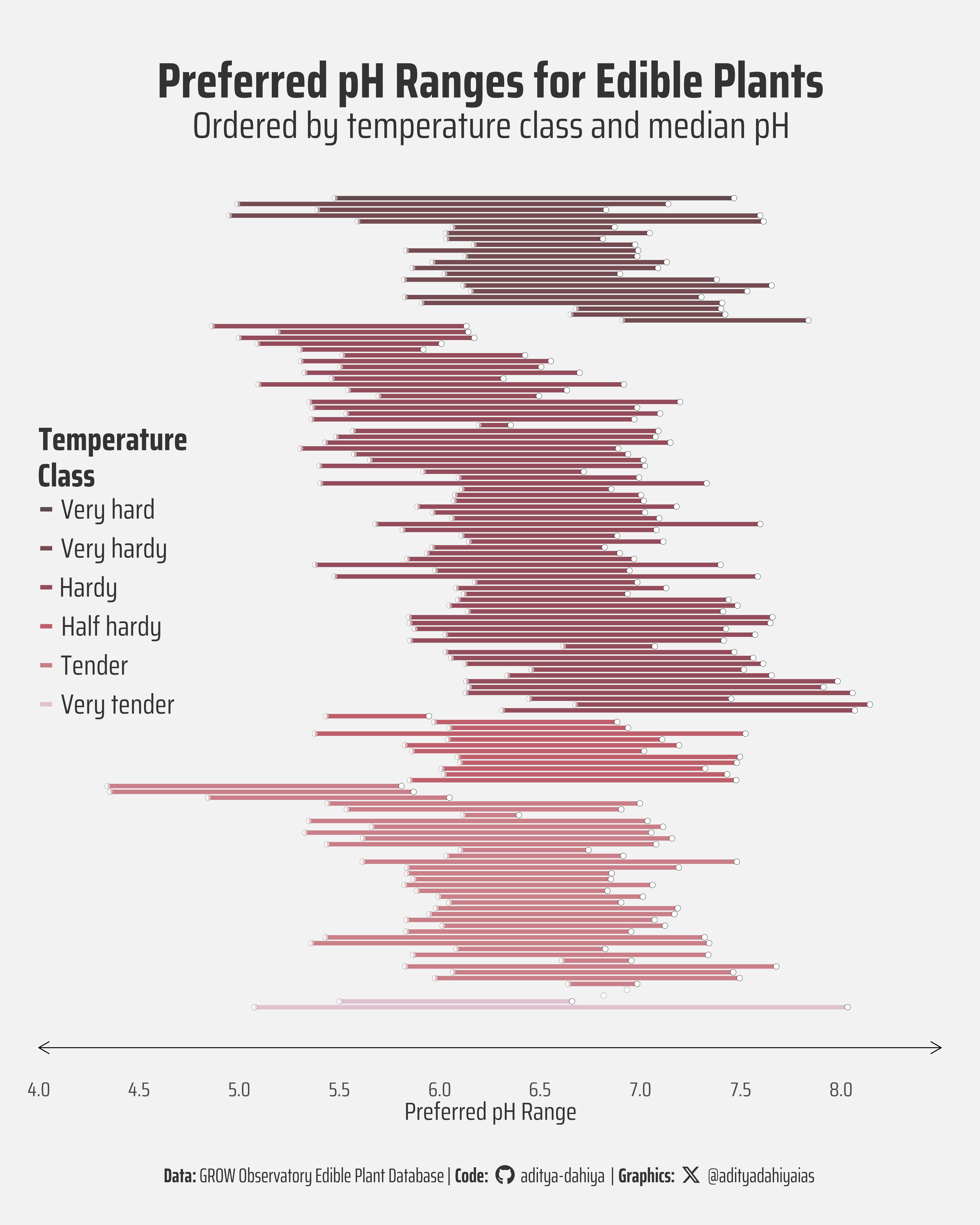
Visualization of preferred pH ranges for plants, ordered by temperature class and median pH preference
#TidyTuesday
Author
Aditya Dahiya
Published
February 4, 2026
About the Data
The Edible Plant Database is a valuable resource that emerged from the GROW Observatory, a European Citizen Science project focused on growing food, soil moisture sensing, and land monitoring. This comprehensive database contains detailed information on 146 edible plant species, including their ideal growing conditions, germination requirements, and time to harvest. The dataset was curated by Nicola Rennie as part of the #TidyTuesday project, a weekly data challenge in the R community. Each entry in the database includes taxonomic and common names, cultivation class, sunlight and water requirements, preferred pH levels, nutrient needs, soil type, growing season, temperature requirements for both germination and growth, time to germination and harvest, nutritional information including energy values, and potential sensitivities or challenges the plant may face. Designed to answer practical questions like “What can I plant now?” and “What can I plant that will yield a crop on a future date?”, this dataset serves as an excellent resource for gardeners, researchers, and data scientists alike to explore relationships between growing conditions and plant characteristics across different geographical locations and seasons.
Figure 1: This visualization reveals the pH preferences of 140 edible plant species from the GROW Observatory database. Each horizontal line represents one plant’s preferred pH range, colored by temperature hardiness. The clustering around pH 6-7 demonstrates that most edible plants thrive in slightly acidic to neutral soil, regardless of their temperature tolerance—a crucial insight for gardeners planning diverse plantings.
How I Made This Graphic
Loading required libraries
Code
pacman::p_load( tidyverse, # All things tidy scales, # Nice Scales for ggplot2 fontawesome, # Icons display in ggplot2 ggtext, # Markdown text support for ggplot2 showtext, # Display fonts in ggplot2 colorspace, # Lighten and Darken colours sf, # Spatial Features patchwork, # Composing Plots packcircles, # for hierarchichal packing circles colorspace, # Modify and play with colours, extract dominant colours magick # Playing with images)edible_plants <- readr::read_csv('https://raw.githubusercontent.com/rfordatascience/tidytuesday/main/data/2026/2026-02-03/edible_plants.csv')
Visualization Parameters
Code
# Font for titlesfont_add_google("Saira",family ="title_font")# Font for the captionfont_add_google("Saira Condensed",family ="body_font")# Font for plot textfont_add_google("Saira Extra Condensed",family ="caption_font")showtext_auto()# A base Colourbg_col <-"grey95"seecolor::print_color(bg_col)# Colour for highlighted texttext_hil <-"grey20"seecolor::print_color(text_hil)# Colour for the texttext_col <-"grey10"seecolor::print_color(text_col)# Define Base Text Sizebts <-120# Caption stuff for the plotsysfonts::font_add(family ="Font Awesome 6 Brands",regular = here::here("docs", "Font Awesome 6 Brands-Regular-400.otf"))github <-""github_username <-"aditya-dahiya"xtwitter <-""xtwitter_username <-"@adityadahiyaias"social_caption_1 <- glue::glue("<span style='font-family:\"Font Awesome 6 Brands\";'>{github};</span> <span style='color: {text_hil}'>{github_username} </span>")social_caption_2 <- glue::glue("<span style='font-family:\"Font Awesome 6 Brands\";'>{xtwitter};</span> <span style='color: {text_hil}'>{xtwitter_username}</span>")plot_caption <-paste0("**Data:** GROW Observatory Edible Plant Database"," | **Code:** ", social_caption_1," | **Graphics:** ", social_caption_2)rm( github, github_username, xtwitter, xtwitter_username, social_caption_1, social_caption_2)plot_title <-"tidy_edible_plants"plot_subtitle <-"ttidy_edible_plants"|>str_wrap(110)
# Define Base Text Size for the plotbts <-90# Improved version with better readability and featuresg <- df1 |>arrange(temperature_class, ph) |>mutate(row_n =row_number()) |>ggplot(aes(y = row_n)) +# Use a single geom_segment with geom_point overlay for cleaner codegeom_segment(aes(x = preferred_ph_lower,xend = preferred_ph_upper,colour = temperature_class ),linewidth =2.4, # Make lines slightly thickeralpha =0.7# Add transparency to see overlaps ) +geom_point(aes(x = preferred_ph_lower),size =3,shape =21,fill ="white",stroke =0.2,alpha =0.5 ) +geom_point(aes(x = preferred_ph_upper),size =3,shape =21,fill ="white",stroke =0.2,alph =0.5 ) + paletteer::scale_colour_paletteer_d("beyonce::X26") +# Improved labels and titleslabs(title ="Preferred pH Ranges for Edible Plants",subtitle ="Ordered by temperature class and median pH",x ="Preferred pH Range",y ="Plant Index",colour ="Temperature\nClass",caption = plot_caption ) +# Extend x-axis slightly for better framingscale_x_continuous(breaks =seq(4, 8, 0.5),limits =c(4, 8.5),expand =expansion(0) ) +scale_y_reverse() +coord_cartesian(clip ="off" ) +theme_minimal(base_family ="body_font",base_size = bts ) +theme(text =element_text(colour ="grey20"),legend.position ="inside",legend.position.inside =c(0, 0.7),legend.justification =c(0, 1),legend.direction ="vertical",legend.text =element_text(margin =margin(3,3,3,3, "mm"),size = bts *1.1 ),legend.title =element_text(margin =margin(0,0,0,0, "mm"),lineheight =0.3,size = bts *1.3,face ="bold" ),legend.margin =margin(0,0,0,0, "mm"),axis.ticks.x.bottom =element_blank(),axis.ticks.length.x.bottom =unit(0, "mm"),panel.grid =element_blank(),axis.line.x =element_line(arrow =arrow(ends ="both",length =unit(5, "mm") ),linewidth =0.5 ),plot.title =element_text(margin =margin(10, 0, 2, 0, "mm"),hjust =0.5,size = bts *2,face ="bold",colour = text_hil ),plot.subtitle =element_text(margin =margin(0, 0, 5, 0, "mm"),hjust =0.5,size = bts *1.5,colour = text_hil ),plot.caption =element_textbox(hjust =0.5,family ="caption_font",size = bts *0.8,colour = text_hil ),axis.text.x =element_text(margin =margin(1,1,1,1, "mm") ),axis.title.x =element_text(margin =margin(1,1,1,1, "mm") ),axis.text.y =element_blank(),axis.title.y =element_blank(),plot.background =element_rect(fill = bg_col, color =NA ) )# Save the plotggsave(filename = here::here("data_vizs","tidy_edible_plants.png" ),plot = g,width =400,height =500,units ="mm",bg = bg_col)
Savings the thumbnail for the webpage
Code
# Saving a thumbnaillibrary(magick)# Saving a thumbnail for the webpageimage_read( here::here("data_vizs","tidy_edible_plants.png" ) ) |>image_resize(geometry ="x400") |>image_write( here::here("data_vizs","thumbnails","tidy_edible_plants.png" ) )
Session Info
Code
pacman::p_load( tidyverse, # All things tidy scales, # Nice Scales for ggplot2 fontawesome, # Icons display in ggplot2 ggtext, # Markdown text support for ggplot2 showtext, # Display fonts in ggplot2 colorspace, # Lighten and Darken colours sf, # Spatial Features patchwork, # Composing Plots packcircles # for hierarchichal packing circles)sessioninfo::session_info()$packages |>as_tibble() |># The attached column is TRUE for packages that were # explicitly loaded with library() dplyr::filter(attached ==TRUE) |> dplyr::select(package,version = loadedversion, date, source ) |> dplyr::arrange(package) |> janitor::clean_names(case ="title" ) |> gt::gt() |> gt::opt_interactive(use_search =TRUE ) |> gtExtras::gt_theme_espn()
Table 1: R Packages and their versions used in the creation of this page and graphics