Mapping Europe’s Elite Basketball Arenas

The Geography of European Basketball Excellence

About the Data

About the Data

This dataset explores EuroLeague Basketball, the top-tier European professional basketball club competition widely regarded as the most prestigious in European basketball. The data includes information on EuroLeague teams such as their country, home city, arena, seating capacity, and historical performance metrics including Final Four appearances and championship titles won. The dataset was curated from publicly available sources including Wikipedia and official EuroLeague records, and is available through the EuroleagueBasketball R package created by Natasa Anastasiadou, with full documentation at natanast.github.io/EuroleagueBasketball. This rich dataset enables exploration of geographic representation across European basketball, comparisons of arena capacities, and analysis of the most historically successful clubs in European basketball competition. The data is part of the #TidyTuesday project, a weekly data visualization challenge in the R and Python communities.

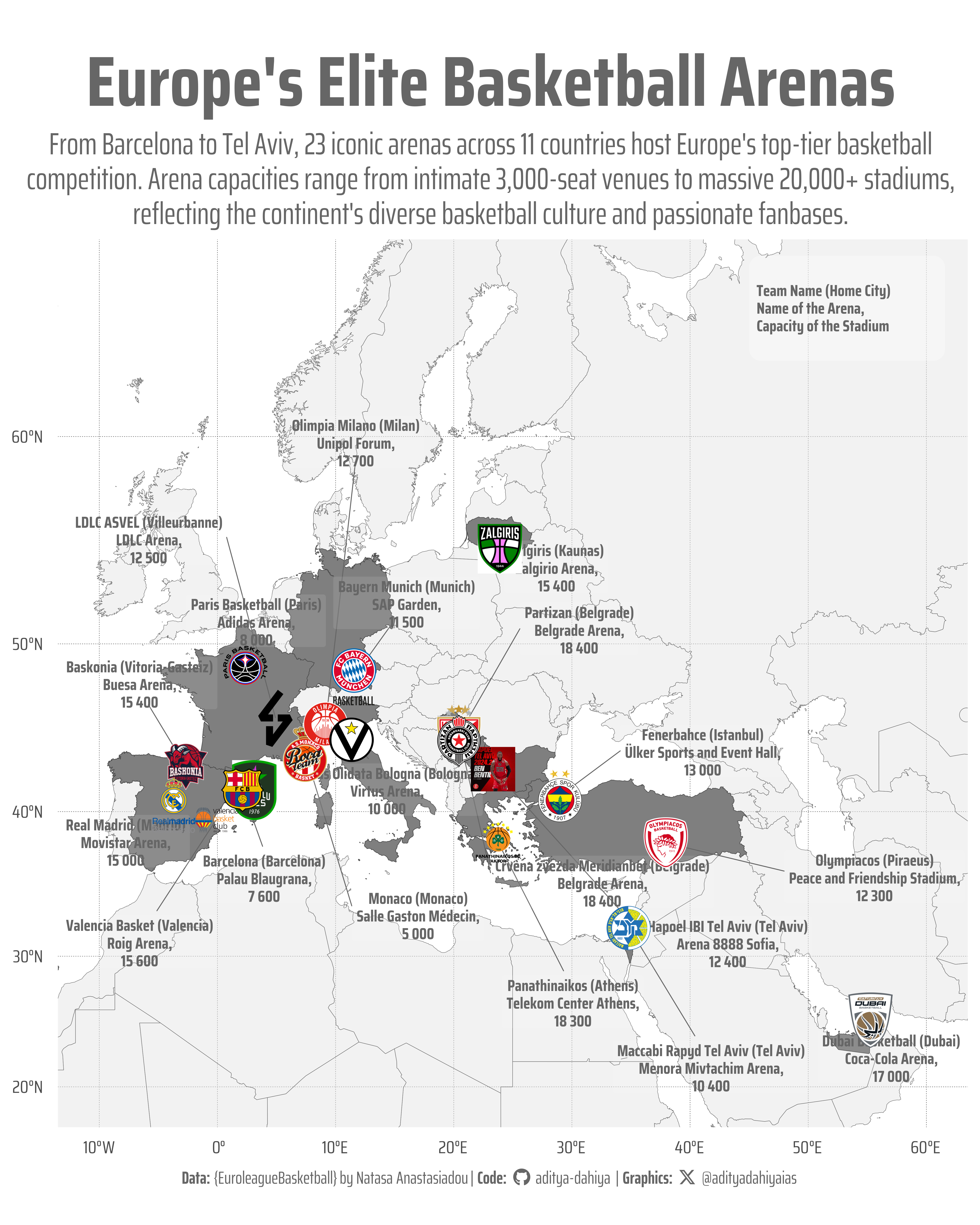
Figure 1: This map visualizes EuroLeague Basketball teams across Europe and beyond, showing arena locations, capacities, and team logos. Created using {ggplot2} with {sf} for spatial data, {ggimage} for team logos, and {ggrepel} for label placement. Map data from {rnaturalearth}, team information from the {EuroleagueBasketball} package. Logos were sourced via Google Custom Search API and processed with {magick}.

How I Made This Graphic

Loading required libraries

pacman::p_load(
  tidyverse, # All things tidy

  scales, # Nice Scales for ggplot2
  fontawesome, # Icons display in ggplot2
  ggtext, # Markdown text support for ggplot2
  showtext, # Display fonts in ggplot2
  colorspace, # Lighten and Darken colours
  sf, # for maps
  patchwork  # Composing Plots
)

euroleague_basketball <- readr::read_csv('https://raw.githubusercontent.com/rfordatascience/tidytuesday/main/data/2025/2025-10-07/euroleague_basketball.csv') |> 
  janitor::clean_names()

Visualization Parameters

# Font for titles
font_add_google("Saira",
  family = "title_font"
)

# Font for the caption
font_add_google("Saira Condensed",
  family = "body_font"
)

# Font for plot text
font_add_google("Saira Extra Condensed",
  family = "caption_font"
)

showtext_auto()

# A base Colour
bg_col <- "white"
seecolor::print_color(bg_col)

# Colour for highlighted text
text_hil <- "grey40"
seecolor::print_color(text_hil)

# Colour for the text
text_col <- "grey30"
seecolor::print_color(text_col)

line_col <- "grey30"

# Define Base Text Size
bts <- 80

# Get the actual colors from chosen palette
day_colors <- paletteer::paletteer_d("ghibli::PonyoDark", n = 7)
names(day_colors) <- c("Sun", "Mon", "Tue", "Wed", "Thu", "Fri", "Sat")

# Caption stuff for the plot
sysfonts::font_add(
  family = "Font Awesome 6 Brands",
  regular = here::here("docs", "Font Awesome 6 Brands-Regular-400.otf")
)
github <- "&#xf09b"
github_username <- "aditya-dahiya"
xtwitter <- "&#xe61b"
xtwitter_username <- "@adityadahiyaias"
social_caption_1 <- glue::glue("<span style='font-family:\"Font Awesome 6 Brands\";'>{github};</span> <span style='color: {text_hil}'>{github_username}  </span>")
social_caption_2 <- glue::glue("<span style='font-family:\"Font Awesome 6 Brands\";'>{xtwitter};</span> <span style='color: {text_hil}'>{xtwitter_username}</span>")
plot_caption <- paste0(
  "**Data:**  {EuroleagueBasketball} by Natasa Anastasiadou",
  " |  **Code:** ",
  social_caption_1,
  " |  **Graphics:** ",
  social_caption_2
)
rm(
  github, github_username, xtwitter,
  xtwitter_username, social_caption_1,
  social_caption_2
)

# Add text to plot-------------------------------------------------
plot_title <- "Europe's Elite Basketball Arenas"

plot_subtitle <- "From Barcelona to Tel Aviv, 23 iconic arenas across 11 countries host Europe's top-tier basketball competition. Arena capacities range from intimate 3,000-seat venues to massive 20,000+ stadiums, reflecting the continent's diverse basketball culture and passionate fanbases." |> 
  str_wrap(100)

str_view(plot_subtitle)

Download images of Club Logos

# Get a custom google search engine and API key
# Tutorial: https://developers.google.com/custom-search/v1/overview
# Tutorial 2: https://programmablesearchengine.google.com/

# From:https://developers.google.com/custom-search/v1/overview
# google_api_key <- "LOAD YOUR GOOGLE API KEY HERE"

# From: https://programmablesearchengine.google.com/controlpanel/all
# my_cx <- "GET YOUR CUSTOM SEARCH ENGINE ID HERE"

pacman::p_load(magick, cropcircles)

# Improved function to download and save food images
download_club_icon <- function(i) {
  
  api_key <- google_api_key
  cx <- my_cx
  
  # Build the API request URL with additional filters
  url <- paste0(
    "https://www.googleapis.com/customsearch/v1?q=",
    URLencode(paste0(euroleague_basketball$team[i], 
                     " basketball logo")),
    "&cx=", cx,
    "&searchType=image",
    "&key=", api_key,
    "&num=1"                 # Fetch only one result
  )
  
  # Make the request
  response <- httr::GET(url)
  if (response$status_code != 200) {
    warning("Failed to fetch data for Cardinal: ", 
            cardinals$name[i])
    return(NULL)
  }
  
  # Parse the response
  result <- httr::content(response, "parsed")
  
  # Extract the image URL
  if (!is.null(result$items)) {
    image_url <- result$items[[1]]$link
  } else {
    warning("No results found for Team: ", euroleague_basketball$team[i])
    return(NULL)
  }
  
  # Process the image
  im <- magick::image_read(image_url) |> 
  #     image_resize("x300") 
  # 
  # # Calculate the new dimension for the square
  # max_dim <- max(image_info(im)$width, image_info(im)$height)
  # 
  # # Create a blank white canvas of square size
  # canvas <- image_blank(width = max_dim, 
  #                       height = max_dim, 
  #                       color = bg_col)
  # 
  # # Composite the original image onto the center of the square canvas
  # image_composite(canvas, im, gravity = "center") |> 
  #   # Crop the image into a circle 
  #   # (Credits: https://github.com/doehm/cropcircles)
  #   cropcircles::circle_crop(
  #     border_colour = text_hil,
  #     border_size = 1
  #   ) |>
  #   image_read() |> 
  #   image_background(color = "transparent") |> 
    image_resize("x300") |>
    # Save or display the result
    image_write(
      here::here(
        "data_vizs", 
        paste0("temp_euroleague_basketball_", i, ".png")
        )
    )
}

# Iterate and download images
for (i in 3:nrow(euroleague_basketball)) {
  download_club_icon(i)
}

Exploratory Data Analysis and Wrangling

# pacman::p_load(summarytools)
# 
# euroleague_basketball |> 
#   dfSummary() |> 
#   view()
# 
# pacman::p_unload(summarytools)

# Get logos of each team

# Source: Claude Sonnet 4.0
# Get the coordinates of each team  city to show on the map
# euroleague_basketball$arena |> paste0(collapse = ", ")
euroleague_arenas <- tibble(
  arena = c(
    "Basketball Development Center",
    "Palau Blaugrana",
    "Buesa Arena",
    "SAP Garden",
    "Belgrade Arena",
    "Coca-Cola Arena",
    "Ülker Sports and Event Hall",
    "Arena 8888 Sofia",
    "Arena Botevgrad",
    "Menora Mivtachim Arena",
    "LDLC Arena",
    "Astroballe",
    "Salle Gaston Médecin",
    "Unipol Forum",
    "Peace and Friendship Stadium",
    "Telekom Center Athens",
    "Adidas Arena",
    "Accor Arena",
    "Movistar Arena",
    "Roig Arena",
    "Virtus Arena",
    "PalaDozza",
    "Žalgirio Arena"
  ),
  longitude = c(
    3.1177,      # Barcelona (Basketball Development Center)
    2.1228,      # Barcelona (Palau Blaugrana)
    -2.6733,     # Vitoria-Gasteiz (Buesa Arena)
    11.5497,     # Munich (SAP Garden)
    20.4289,     # Belgrade (Belgrade Arena)
    55.2708,     # Dubai (Coca-Cola Arena)
    29.0275,     # Istanbul (Ülker Sports and Event Hall)
    23.3219,     # Sofia (Arena 8888 Sofia)
    23.7833,     # Botevgrad (Arena Botevgrad)
    34.8116,     # Tel Aviv (Menora Mivtachim Arena)
    4.9267,      # Villeurbanne (LDLC Arena)
    4.9267,      # Villeurbanne (Astroballe)
    7.4167,      # Monaco (Salle Gaston Médecin)
    9.1497,      # Milan (Unipol Forum)
    37.9475,     # Piraeus (Peace and Friendship Stadium)
    23.7514,     # Athens (Telekom Center Athens)
    2.3522,      # Paris (Adidas Arena)
    2.3792,      # Paris (Accor Arena)
    -3.6753,     # Madrid (Movistar Arena)
    -0.1058,     # Valencia (Roig Arena)
    11.3514,     # Bologna (Virtus Arena)
    11.3428,     # Bologna (PalaDozza)
    23.9036      # Kaunas (Žalgirio Arena)
  ),
  latitude = c(
    41.3806,     # Barcelona (Basketball Development Center)
    41.3809,     # Barcelona (Palau Blaugrana)
    42.8520,     # Vitoria-Gasteiz (Buesa Arena)
    48.1756,     # Munich (SAP Garden)
    44.7769,     # Belgrade (Belgrade Arena)
    25.2048,     # Dubai (Coca-Cola Arena)
    41.0392,     # Istanbul (Ülker Sports and Event Hall)
    42.6977,     # Sofia (Arena 8888 Sofia)
    42.9000,     # Botevgrad (Arena Botevgrad)
    32.1133,     # Tel Aviv (Menora Mivtachim Arena)
    45.7667,     # Villeurbanne (LDLC Arena)
    45.7667,     # Villeurbanne (Astroballe)
    43.7384,     # Monaco (Salle Gaston Médecin)
    45.4375,     # Milan (Unipol Forum)
    37.9475,     # Piraeus (Peace and Friendship Stadium)
    37.9838,     # Athens (Telekom Center Athens)
    48.8566,     # Paris (Adidas Arena)
    48.8394,     # Paris (Accor Arena)
    40.4168,     # Madrid (Movistar Arena)
    39.4699,     # Valencia (Roig Arena)
    44.4949,     # Bologna (Virtus Arena)
    44.4938,     # Bologna (PalaDozza)
    54.8985      # Kaunas (Žalgirio Arena)
  ),
  iso_a2 = c(
    "ES",  # Spain
    "ES",  # Spain
    "ES",  # Spain
    "DE",  # Germany
    "RS",  # Serbia
    "AE",  # United Arab Emirates
    "TR",  # Turkey
    "BG",  # Bulgaria
    "BG",  # Bulgaria
    "IL",  # Israel
    "FR",  # France
    "FR",  # France
    "MC",  # Monaco
    "IT",  # Italy
    "GR",  # Greece
    "GR",  # Greece
    "FR",  # France
    "FR",  # France
    "ES",  # Spain
    "ES",  # Spain
    "IT",  # Italy
    "IT",  # Italy
    "LT"   # Lithuania
  )
) |> 
  st_as_sf(coords = c("longitude", "latitude"), crs = 4326, remove = FALSE)

df1 <- euroleague_arenas |> 
  left_join(
    euroleague_basketball |> 
      mutate(image_id = row_number()) |> 
      separate_longer_delim(
        cols = arena,
        delim = " \\ "
      ) |> 
      separate_longer_delim(
        cols = arena,
        delim = ", "
      ) |>
      mutate(
        arena = str_trim(arena)
    )
  ) |> 
  # First, separate rows that have two capacities (separated by comma and space)
  separate_longer_delim(capacity, delim = ", ") %>%
  # Parse as numbers (remove commas and convert to numeric)
  mutate(capacity = parse_number(capacity)) |> 
  group_by(team) |> 
  slice_head(n = 1) |> 
  ungroup() |> 
  st_as_sf()

world_map <- rnaturalearth::ne_countries(
      returnclass = "sf",
      scale = "large"
    ) |> 
      select(iso_a2, geometry)

country_map <- df1 |> 
  st_drop_geometry() |> 
  select(iso_a2) |> 
  left_join(
    rnaturalearth::ne_countries(
      returnclass = "sf",
      scale = "large"
    ) |> 
      select(name, iso_a2, geometry) |> 
  mutate(
    iso_a2 = if_else(
      iso_a2 == "-99" & name == "France", 
      "FR", 
      iso_a2)
    )
  ) |> 
  st_as_sf()

The Plot

g <- ggplot() +
  geom_sf(
    data = world_map,
    fill = "grey90",
    colour = text_hil,
    linewidth = 0.2,
    alpha = 0.5
  ) +
  geom_sf(
    data = country_map,
    fill = "grey50",
    colour = text_col,
    linewidth = 0.3
  ) +

  # Replace the geom_label_repel with:
  ggrepel::geom_label_repel(
      data = df1,
      mapping = aes(
        label = paste0(
          team, " (", home_city, ") \n",
          arena, ", ", "\n",
          number(capacity, accuracy = 100)
        ),
        geometry = geometry
      ),
      stat = "sf_coordinates",
      hjust = 0.5,
      vjust = 0,
      lineheight = 0.3,
      family = "body_font",
      fill = alpha("white", 0.1),
      label.size = NA,
      label.r = unit(0.2, "lines"),
      label.padding = unit(0.25, "lines"),
      force_pull = 0.01,
      force = 200,
      seed = 21,
      size = bts / 4,
      colour = text_hil,
      fontface = "bold",
      min.segment.length = unit(1, "mm")
    ) +
     ggimage::geom_image(
      data = df1,
      mapping = aes(
          x = longitude, 
          y = latitude, 
          image = paste0("data_vizs/temp_euroleague_basketball_", image_id, ".png")
        ),
        size = 0.05
      ) +
    # Add legend annotation
    annotate(
      geom = "label",
      x = 45, 
      y = 65,
      label = paste0(
          "Team Name", " (Home City) \n",
          "Name of the Arena, ", "\n",
          "Capacity of the Stadium"
        ),
      family = "body_font",
      fill = alpha("white", 0.3),
      label.size = NA,
      label.r = unit(0.2, "lines"),
      label.padding = unit(0.5, "lines"),
      hjust = 0,
      vjust = 0.5,
      lineheight = 0.3,
      size = bts / 4,
      colour = text_hil,
      fontface = "bold"
  ) +

  coord_sf(
    crs = "EPSG:3857",
    default_crs = "EPSG:4326",
    xlim = c(-10, 60),
    ylim = c(20, 66)
  ) +
  
  labs(
    title = plot_title,
    subtitle = plot_subtitle,
    caption = plot_caption,
    colour = NULL,
    fill = NULL,
    x = NULL, y = NULL
  ) +
  theme_minimal(
    base_family = "body_font",
    base_size = bts
  ) +
  theme(
    legend.position = "none",
    
    # Overall
    text = element_text(
      margin = margin(0, 0, 0, 0, "mm"),
      colour = text_col,
      lineheight = 0.3
    ),
    
    # Grid Lines and Axes Text
    panel.grid = element_line(
      linewidth = 0.3,
      linetype = 3,
      colour = text_hil
    ),
    axis.text = element_text(
      margin = margin(0,0,0,0, "mm")
    ),
    axis.ticks.length = unit(0, "mm"),
    
    # Labels and Strip Text
    plot.title = element_text(
      margin = margin(5, 0, 5, 0, "mm"),
      hjust = 0.5,
      vjust = 0.5,
      colour = text_hil,
      size = 3.2 * bts,
      family = "body_font",
      face = "bold",
      lineheight = 0.25
    ),
    plot.subtitle = element_text(
      margin = margin(2, 0, 5, 0, "mm"),
      vjust = 0.5,
      colour = text_hil,
      size = 1.4 * bts,
      hjust = 0.5,
      family = "caption_font",
      lineheight = 0.3
    ),
    plot.caption = element_markdown(
      family = "caption_font",
      hjust = 0.5,
      margin = margin(5,0,0,0, "mm"),
      colour = text_hil
    ),
    plot.caption.position = "plot",
    plot.title.position = "plot",
    plot.margin = margin(5, 5, 5, 5, "mm")
  )

ggsave(
  filename = here::here(
    "data_vizs",
    "tidy_euroleague_basketball.png"
  ),
  plot = g,
  width = 400,
  height = 500,
  units = "mm",
  bg = bg_col
)

Savings the thumbnail for the webpage

# Saving a thumbnail

library(magick)

# Saving a thumbnail for the webpage
image_read(here::here(
  "data_vizs",
  "tidy_euroleague_basketball.png"
)) |>
  image_resize(geometry = "x400") |>
  image_write(
    here::here(
      "data_vizs",
      "thumbnails",
      "tidy_euroleague_basketball.png"
    )
  )

Session Info

sessioninfo::session_info()$packages |>
  as_tibble() |>
  dplyr::select(package,
    version = loadedversion,
    date, source
  ) |>
  dplyr::arrange(package) |>
  janitor::clean_names(
    case = "title"
  ) |>
  gt::gt() |>
  gt::opt_interactive(
    use_search = TRUE
  ) |>
  gtExtras::gt_theme_espn()

Table 1: R Packages and their versions used in the creation of this page and graphics

Links

• Wikipedia
• official EuroLeague records
• EuroleagueBasketball R package
• Natasa Anastasiadou
• natanast.github.io/EuroleagueBasketball
• #TidyTuesday