The James Beard Awards - Nominees and Awardees

Stacked Bar charts, adding logo (images from {magick}) to ggplot2, using {ggpattern} and extracting a colour palette from an image.

About the Data

The James Beard Awards dataset provides an in-depth look at the annual awards recognizing excellence in culinary arts, journalism, and leadership within the United States. This dataset, curated by Jon Harmon and suggested by PythonCoderUnicorn, includes multiple facets of the awards spanning categories such as books, broadcast media, journalism, leadership, and restaurants and chefs. Each dataset captures variables such as award rank, year, subcategory, and affiliations, offering rich opportunities for analysis. Users can access these datasets via the tidytuesdayR package or directly from GitHub. Explore how award subcategories evolved over time, identify multi-category winners, and analyze prominent affiliations in culinary and media landscapes.

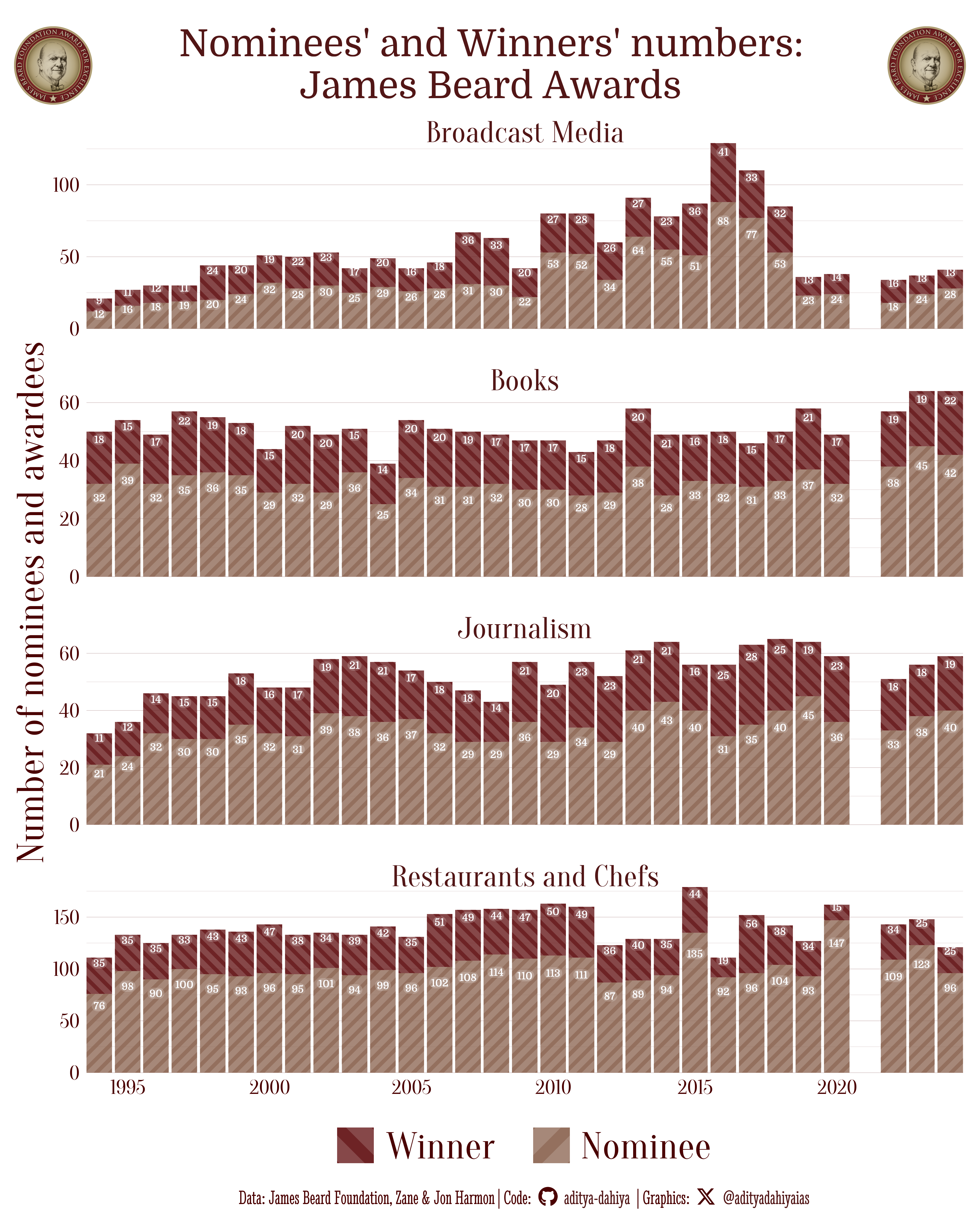
Figure 1: A bar chart showing the number of nominees and awardees under 4 different categories of the James Beard Awards. The {ggimage} has been used to add logos to the graphic, and the {imgpalr} has been used to generate a colour palette from the logo, to be used in the graphic.

How I made this graphic?

Loading required libraries, data import & creating custom functions. Downloading the logo.

# Data Import and Wrangling Tools
library(tidyverse)            # All things tidy

# Final plot tools
library(scales)               # Nice Scales for ggplot2
library(fontawesome)          # Icons display in ggplot2
library(ggtext)               # Markdown text support for ggplot2
library(showtext)             # Display fonts in ggplot2
library(colorspace)           # Lighten and Darken colours
library(patchwork)            # Compiling Plots
library(imgpalr)              # Extracting palettes from images

# Option 2: Read directly from GitHub
book <- readr::read_csv('https://raw.githubusercontent.com/rfordatascience/tidytuesday/main/data/2024/2024-12-31/book.csv')
broadcast_media <- readr::read_csv('https://raw.githubusercontent.com/rfordatascience/tidytuesday/main/data/2024/2024-12-31/broadcast_media.csv')
journalism <- readr::read_csv('https://raw.githubusercontent.com/rfordatascience/tidytuesday/main/data/2024/2024-12-31/journalism.csv')
leadership <- readr::read_csv('https://raw.githubusercontent.com/rfordatascience/tidytuesday/main/data/2024/2024-12-31/leadership.csv')
restaurant_and_chef <- readr::read_csv('https://raw.githubusercontent.com/rfordatascience/tidytuesday/main/data/2024/2024-12-31/restaurant_and_chef.csv')

# Get image logo of James Beard Awards
url <- "https://imageio.forbes.com/blogs-images/johnmariani/files/2019/03/jb-medal-1200x1200.png"
logo1 <- magick::image_read(url) |> 
  magick::image_resize("x400")

Visualization Parameters. Extracting colour palette.

# Font for titles
font_add_google("Domine",
  family = "title_font"
) 

# Font for the caption
font_add_google("Stint Ultra Condensed",
  family = "caption_font"
) 

# Font for plot text
font_add_google("Oranienbaum",
  family = "body_font"
) 

showtext_auto()

# Extract a colour palette from an image
# set.seed(1)
# magick::image_write(
#   logo1,
#   path = here::here("data", "temp_tidy_james_beard_awards.png")
# )
# mypal <- imgpalr::image_pal(
#   file = here::here("data", "temp_tidy_james_beard_awards.png"),
#   n = 7
# )
# unlink(here::here("data", "temp_tidy_james_beard_awards.png"))

mypal <- c("#A68D6F", "#906A57", "#FCFCFE", 
           "#521616", "#681A1C", "#7B473D",
           "#A7976F")
mypal |> 
  seecolor::print_color()

# A base Colour
bg_col <- mypal[3]
seecolor::print_color(bg_col)

# Colour for highlighted text
text_hil <- mypal[4]
seecolor::print_color(text_hil)

# Colour for the text
text_col <- colorspace::darken(mypal[4], 0.3)
seecolor::print_color(text_col)


# Define Base Text Size
bts <- 90 

# Caption stuff for the plot
sysfonts::font_add(
  family = "Font Awesome 6 Brands",
  regular = here::here("docs", "Font Awesome 6 Brands-Regular-400.otf")
)
github <- "&#xf09b"
github_username <- "aditya-dahiya"
xtwitter <- "&#xe61b"
xtwitter_username <- "@adityadahiyaias"
social_caption_1 <- glue::glue("<span style='font-family:\"Font Awesome 6 Brands\";'>{github};</span> <span style='color: {text_hil}'>{github_username}  </span>")
social_caption_2 <- glue::glue("<span style='font-family:\"Font Awesome 6 Brands\";'>{xtwitter};</span> <span style='color: {text_hil}'>{xtwitter_username}</span>")
plot_caption <- paste0(
  "**Data:** James Beard Foundation, Zane & Jon Harmon ", 
  " |  **Code:** ", 
  social_caption_1, 
  " |  **Graphics:** ", 
  social_caption_2
  )
rm(github, github_username, xtwitter, 
   xtwitter_username, social_caption_1, 
   social_caption_2)

# Add text to plot-------------------------------------------------
plot_title <- "Nominees' and Winners' numbers:\nJames Beard Awards"

plot_subtitle <- "Over the last 3 decades, nominees and winners in different categories has varied. There were no awards in 2021."

Exploratory Data Analysis and Wrangling

# Lets look at the years range for each data set
# book$year |> range()
# broadcast_media$year |> range()
# journalism$year |> range()
# restaurant_and_chef$year |> range()
# leadership$year |> range()

clean_up <- function(data1, text1){
  data1 |> 
  filter(year > 1993) |> 
  count(year, rank) |>
  mutate(class = text1)
}

df <- rbind(
  clean_up(book, "Books"),
  clean_up(broadcast_media, "Broadcast Media"),
  clean_up(journalism, "Journalism"),
  clean_up(restaurant_and_chef, "Restaurants and Chefs")
) |> 
  filter(rank %in% c("Nominee", "Winner")) |> 
  mutate(
    rank = fct(rank, levels = c("Winner", "Nominee")),
    class = fct(
      class, 
      levels = c(
        "Broadcast Media",
        "Books",
        "Journalism",
        "Restaurants and Chefs"
      )
    )
  )

The Base Plot, using {ggpattern}

library(ggpattern)

g1 <- df |> 
  ggplot(
    mapping = aes(
      x = year,
      y = n
    )
  ) +
  # Actual data displayed in the graphic
  ggpattern::geom_col_pattern(
    mapping = aes(
      fill = rank,
      pattern_angle = rank,
      pattern_fill = rank
    ),
    position = position_stack(),
    pattern = "stripe",
    pattern_density = 0.4,
    pattern_colour = "transparent"
  ) +
  geom_label(
    mapping = aes(
      label = n
    ),
    fill = alpha("white", 0.2),
    position = position_stack(
      vjust = 0.85
    ),
    family = "title_font",
    size = bts / 7,
    fontface = "bold",
    colour = bg_col,
    label.r = unit(0.15, "lines"),
    label.padding = unit(0.05, "lines"),
    label.size = NA
  ) +
  # Scales and Coordinates
  scale_fill_manual(
    values = c(alpha(mypal[5], 0.8), alpha(mypal[2], 0.8))
  ) +
  scale_pattern_fill_manual(
    values = c(alpha(mypal[5], 0.8), alpha(mypal[2], 0.8))
  ) +
  scale_pattern_angle_manual(
    values = c(-45, 45)
  ) +
  scale_x_continuous(
    expand = expansion(0),
    breaks = seq(1995, 2024, 5)
  ) +
  scale_y_continuous(
    expand = expansion(c(0, 0.05))
  ) +
  coord_cartesian(
    clip = "off"
  ) +
  
  # Facets
  facet_wrap(
    ~class,
    ncol = 1,
    scales = "free_y"
  ) +
  
  # Labels and Themes
  labs(
    x = NULL, 
    y = "Number of nominees and awardees",
    fill = NULL,
    pattern_fill = NULL,
    pattern_angle = NULL,
    title = plot_title,
    subtitle = NULL,
    caption = plot_caption
  ) +
  theme_minimal(
    base_family = "body_font",
    base_size = bts
  ) +
  theme(
    # Overall plot
    plot.margin = margin(5,5,5,5, "mm"),
    plot.title.position = "plot",
    text = element_text(
      colour = text_col,
      margin = margin(0,0,0,0, "mm"),
      
    ),
    
    # Axes
    axis.ticks = element_blank(),
    axis.ticks.length = unit(0, "mm"),
    axis.text.x = element_text(
      margin = margin(3,0,0,0, "mm"),
      colour = text_col
    ),
    axis.text.y = element_text(
      margin = margin(0,3,0,0, "mm"),
      colour = text_col
    ),
    axis.title.y = element_text(
      margin = margin(0,0,0,0, "mm"),
      size = 1.5 * bts
    ),
    
    # Panel
    panel.grid.major.x = element_blank(),
    panel.grid.minor.x = element_blank(),
    panel.grid.major.y = element_line(
      colour = alpha(text_col, 0.4),
      linewidth = 0.15
    ),
    panel.grid.minor.y = element_line(
      colour = alpha(text_col, 0.4),
      linewidth = 0.08
    ),
    
    # Strip Text and Facets
    panel.spacing.y = unit(15, "mm"),
    strip.text = element_text(
      hjust = 0.5,
      margin = margin(0,0,-5,0, "mm"),
      size = 1.2 * bts,
      colour = text_hil
    ),
    
    # Legend 
    legend.position = "bottom",
    legend.direction = "horizontal",
    legend.text = element_text(
      margin = margin(0,0,0,5, "mm"),
      size = 1.5 * bts
    ),
    legend.key.height = unit(7, "mm"),
    legend.key.width = unit(15, "mm"),
    legend.margin = margin(-20,0,10,0, "mm"),
    legend.box.margin = margin(0,0,0,0, "mm"),
    
    # Labels
    plot.title = element_text(
      size = 1.5 * bts,
      margin = margin(5,0,5,0, "mm"),
      hjust = 0.5,
      family = "title_font",
      colour = text_hil,
      lineheight = 0.3
    ),
    plot.subtitle = element_text(
      margin = margin(0,0,0,0, "mm"),
      hjust = 1,
      colour = text_hil,
      lineheight = 0.3
    ),
    plot.caption = element_textbox(
      family = "caption_font",
      hjust = 0.5,
      margin = margin(0,0,0,0, "mm")
    )
    
  )

inset1 <- ggplot() +
  annotation_custom(
    grob = grid::rasterGrob(logo1),
    xmin = 0, xmax = 1,
    ymin = 0, ymax = 1
  ) +
  theme_void() +
  theme(
    plot.background = element_rect(
      fill = "transparent", colour = "transparent"
    ),
    panel.background = element_rect(
      fill = "transparent", colour = "transparent"
    )
  )

g <- g1 +
  inset_element(
    p = inset1,
    on_top = TRUE,
    ignore_tag = TRUE,
    clip = FALSE,
    align_to = "full",
    left = 0, right = 0.1,
    bottom = 0.9, top = 1
  ) +
  inset_element(
    p = inset1,
    on_top = TRUE,
    ignore_tag = TRUE,
    clip = FALSE,
    align_to = "full",
    left = 0.9, right = 1,
    bottom = 0.9, top = 1
  )

ggsave(
  filename = here::here(
    "data_vizs",
    "tidy_james_beard_awards.png"
  ),
  plot = g,
  width = 400,
  height = 500,
  units = "mm",
  bg = bg_col
)

Savings the thumbnail for the webpage

# Saving a thumbnail

library(magick)
# Saving a thumbnail for the webpage
image_read(here::here("data_vizs", 
                      "tidy_james_beard_awards.png")) |> 
  image_resize(geometry = "x400") |> 
  image_write(
    here::here(
      "data_vizs", 
      "thumbnails", 
      "tidy_james_beard_awards.png"
    )
  )

Session Info

# Data Import and Wrangling Tools
library(tidyverse)            # All things tidy

# Final plot tools
library(scales)               # Nice Scales for ggplot2
library(fontawesome)          # Icons display in ggplot2
library(ggtext)               # Markdown text support for ggplot2
library(showtext)             # Display fonts in ggplot2
library(colorspace)           # Lighten and Darken colours
library(patchwork)            # Compiling Plots

sessioninfo::session_info()$packages |> 
  as_tibble() |> 
  select(package, 
         version = loadedversion, 
         date, source) |> 
  arrange(package) |> 
  janitor::clean_names(
    case = "title"
  ) |> 
  gt::gt() |> 
  gt::opt_interactive(
    use_search = TRUE
  ) |> 
  gtExtras::gt_theme_espn()

Table 1: R Packages and their versions used in the creation of this page and graphics