A circle-packed visualization of linguistic diversity at risk across six macroareas
#TidyTuesday
{packcircles}
Circle Visualization
Author
Aditya Dahiya
Published
December 27, 2025
About the Data
This dataset explores the world’s languages using data from Glottolog 5.2.1, the most comprehensive language database in linguistics. Maintained by the Max Planck Institute for Evolutionary Anthropology, Glottolog contains detailed information on over 8,000 languages worldwide, including names, genealogy, geographical distributions, and endangerment status. The dataset comprises three interconnected tables: languages.csv provides core information about each language including geographic coordinates, ISO 639-3 codes, macroarea classifications, and whether the language is an isolate with no known relatives; families.csv catalogs the language families to which non-isolate languages belong; and endangered_status.csv documents the endangerment status of languages using a six-category classification system. This rich dataset enables exploration of fascinating questions about linguistic diversity, such as which regions have the highest concentrations of endangered languages, whether language isolates face greater endangerment risks, and how language families are distributed geographically across the globe. The data was curated by Darakhshan Nehal for #TidyTuesday, a weekly data project in the R for Data Science online learning community.
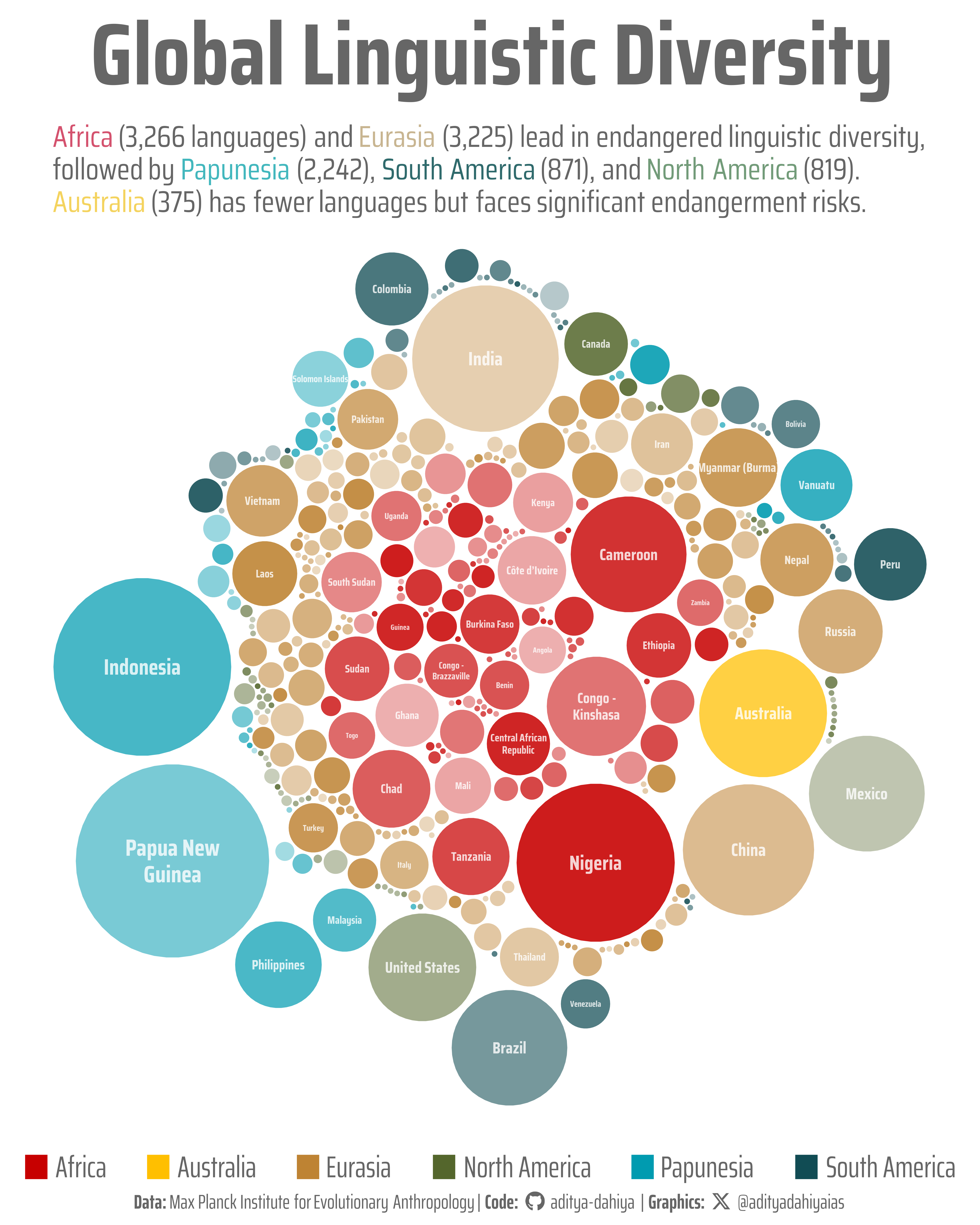
Figure 1: This visualization maps the distribution of endangered languages across countries and macroareas worldwide. Each circle represents a country, with size proportional to the number of endangered languages it contains. Countries are colored by their macroarea—the broad geographic region they belong to—revealing distinct patterns of linguistic endangerment. Africa (red) and Papunesia (teal) show particularly high concentrations, with Nigeria and Indonesia harboring the most endangered languages. The varying transparency of circles adds visual depth while highlighting the complex, overlapping nature of global linguistic diversity under threat.
How I Made This Graphic
.
Loading required libraries
Code
pacman::p_load( tidyverse, # All things tidy scales, # Nice Scales for ggplot2 fontawesome, # Icons display in ggplot2 ggtext, # Markdown text support for ggplot2 showtext, # Display fonts in ggplot2 colorspace, # Lighten and Darken colours sf, # Spatial Features patchwork, # Composing Plots packcircles # for hierarchichal packing circles)endangered_status <- readr::read_csv('https://raw.githubusercontent.com/rfordatascience/tidytuesday/main/data/2025/2025-12-23/endangered_status.csv')families <- readr::read_csv('https://raw.githubusercontent.com/rfordatascience/tidytuesday/main/data/2025/2025-12-23/families.csv')languages <- readr::read_csv('https://raw.githubusercontent.com/rfordatascience/tidytuesday/main/data/2025/2025-12-23/languages.csv')world <- rnaturalearth::ne_countries(returnclass ="sf")
Visualization Parameters
Code
# Font for titlesfont_add_google("Saira",family ="title_font")# Font for the captionfont_add_google("Saira Condensed",family ="body_font")# Font for plot textfont_add_google("Saira Extra Condensed",family ="caption_font")showtext_auto()# A base Colourbg_col <-"white"seecolor::print_color(bg_col)# Colour for highlighted texttext_hil <-"grey40"seecolor::print_color(text_hil)# Colour for the texttext_col <-"grey30"seecolor::print_color(text_col)line_col <-"grey30"# Define Base Text Sizebts <-80mypal <- paletteer::paletteer_d("ltc::trio3")[c(2, 3, 1)]# Caption stuff for the plotsysfonts::font_add(family ="Font Awesome 6 Brands",regular = here::here("docs", "Font Awesome 6 Brands-Regular-400.otf"))github <-""github_username <-"aditya-dahiya"xtwitter <-""xtwitter_username <-"@adityadahiyaias"social_caption_1 <- glue::glue("<span style='font-family:\"Font Awesome 6 Brands\";'>{github};</span> <span style='color: {text_hil}'>{github_username} </span>")social_caption_2 <- glue::glue("<span style='font-family:\"Font Awesome 6 Brands\";'>{xtwitter};</span> <span style='color: {text_hil}'>{xtwitter_username}</span>")plot_caption <-paste0("**Data:** Max Planck Institute for Evolutionary Anthropology"," | **Code:** ", social_caption_1," | **Graphics:** ", social_caption_2)rm( github, github_username, xtwitter, xtwitter_username, social_caption_1, social_caption_2)plot_title <-"Global Linguistic Diversity"plot_subtitle <-"<span style='color:#D4526E'>Africa</span> (3,266 languages) and <span style='color:#C8B591'>Eurasia</span> (3,225) lead in endangered linguistic diversity,<br>followed by <span style='color:#42B7BD'>Papunesia</span> (2,242), <span style='color:#2F6A6C'>South America</span> (871), and <span style='color:#729B79'>North America</span> (819).<br><span style='color:#F4D35E'>Australia</span> (375) has fewer languages but faces significant endangerment risks."
Exploratory Data Analysis and Wrangling
Code
bts =80plotdf <- languages |>select(id, name, countries, macroarea) |>left_join(endangered_status) |>select(-status_code) |>drop_na() |>separate_longer_delim(cols = countries, ";") |>separate_longer_delim(cols = macroarea, ";") |>count(macroarea, countries) |>mutate(countries =str_to_lower(countries),country = countrycode::countrycode(sourcevar = countries,origin ="iso2c",destination ="country.name.en" ),country =str_wrap(country, 15) )plotdf <- plotdf |>mutate(alpha_var =runif(nrow(plotdf)))# endangered_status |> # count(status_label)# # languages |> # drop_na(longitude, latitude) |> # st_as_sf(# coords = c("longitude", "latitude"),# crs = "EPSG:4326"# ) |> # ggplot() +# geom_sf(data = world) +# geom_sf()# Prepare data for circle packing# Need to create a proper hierarchy with groups and subgroupspacking_data <- plotdf |>select(macroarea, country, n, alpha_var) |>mutate(group = macroarea,subgroup = country,value = n )# Create the packing layout# First, we need to format data for circleProgressiveLayoutpacking <-circleProgressiveLayout(packing_data$value, sizetype ='area')packing$radius <-0.95* packing$radius # Add some spacing# Add packing coordinates back to datapacking_data <-bind_cols(packing_data, packing)# Generate circle coordinates for plottingcircle_data <-circleLayoutVertices(packing, npoints =50)# Join back the grouping informationcircle_data <- circle_data |>left_join( packing_data |>mutate(id =row_number()) |>select(id, group, subgroup, value, alpha_var),by ="id" )# plotdf |> # group_by(macroarea) |> # summarise(n = sum(n))
# Saving a thumbnaillibrary(magick)# Saving a thumbnail for the webpageimage_read(here::here("data_vizs","tidy_languages_world.png")) |>image_resize(geometry ="x400") |>image_write( here::here("data_vizs","thumbnails","tidy_languages_world.png" ) )
Session Info
Code
pacman::p_load( tidyverse, # All things tidy scales, # Nice Scales for ggplot2 fontawesome, # Icons display in ggplot2 ggtext, # Markdown text support for ggplot2 showtext, # Display fonts in ggplot2 colorspace, # Lighten and Darken colours sf, # Spatial Features patchwork, # Composing Plots packcircles # for hierarchichal packing circles)sessioninfo::session_info()$packages |>as_tibble() |># The attached column is TRUE for packages that were # explicitly loaded with library() dplyr::filter(attached ==TRUE) |> dplyr::select(package,version = loadedversion, date, source ) |> dplyr::arrange(package) |> janitor::clean_names(case ="title" ) |> gt::gt() |> gt::opt_interactive(use_search =TRUE ) |> gtExtras::gt_theme_espn()
Table 1: R Packages and their versions used in the creation of this page and graphics