Tracking Mt. Vesuvius: Seismic Centroids on the Move

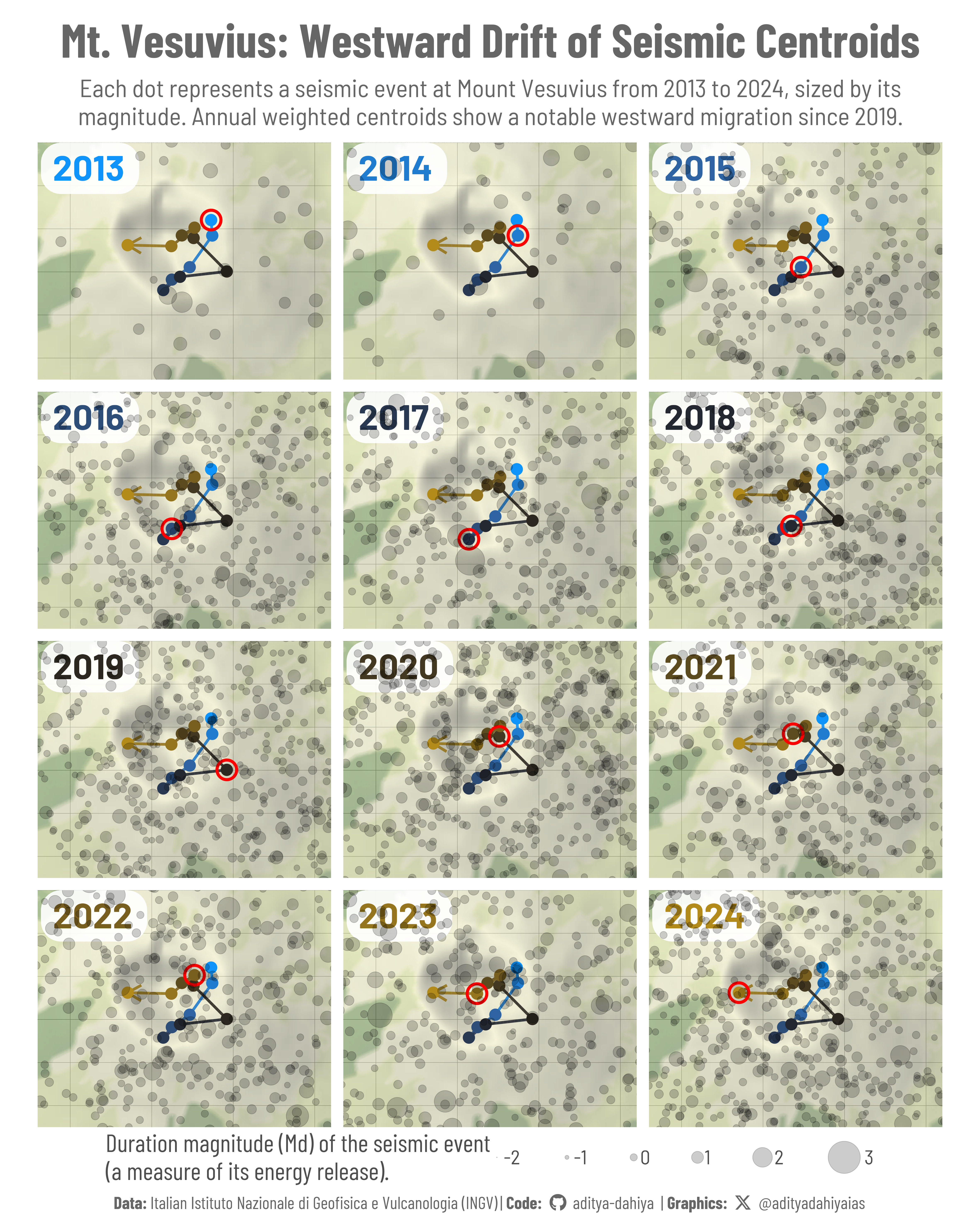
The graphic highlights a subtle but consistent westward shift in the center of seismic activity at Mount Vesuvius over the past decade.

About the Data

This dataset captures seismic activity at Mount Vesuvius, one of the most iconic and closely monitored volcanoes in the world, located in Campania, Italy. The data originates from the Istituto Nazionale di Geofisica e Vulcanologia (INGV), Italy’s national institute for geophysics and volcanology, and is accessible through its Open Data Portal. The specific dataset was curated from the GOSSIP portal, which offers interactive access to seismic records for various volcanic regions. Originally available as individual CSV files in Italian, the dataset was consolidated and partially translated into English for broader usability. It includes variables such as the event’s date, time, location, depth, magnitude, and classification (e.g., earthquake or eruption), with metadata indicating the quality and review level of each observation. This dataset was featured in the #TidyTuesday project for the week of May 13, 2025, and made available for analysis in R, Python, and Julia. Special thanks to Libby Heeren for curating and sharing this valuable resource for public exploration and visualization.

Figure 1: This graphic shows the geographic distribution of seismic events at Mount Vesuvius from 2013 to 2024, with each earthquake represented as a grey dot sized by its duration magnitude (Md). For each year, the red circle marks the weighted centroid of all events, calculated using Md as the weighting factor. Over the 12-year period, the centroids trace a clear westward shift beginning in 2019, suggesting a possible geographic migration of seismic activity within the region. This trend may warrant further investigation into evolving subsurface dynamics at the volcano.

How the Graphic Was Created

To visualize the westward migration of seismic activity near Mount Vesuvius, I used the tidyverse suite for data wrangling and ggplot2 for plotting. Earthquake data were obtained via readr::read_csv(), and weighted centroids by year were computed using dplyr::summarise() with weighted.mean(). A background terrain map was retrieved using ggmap::get_stadiamap() and layered with terra::rast(). The final plot includes yearly earthquake points sized by duration_magnitude_md, annual centroid paths (geom_path()), and highlighted centroids (geom_point() and geom_label()) using a diverging color scale from paletteer. The plot was styled with custom fonts via showtext and exported using ggsave().

Loading required libraries

pacman::p_load(
  tidyverse,            # All things tidy
  
  scales,               # Nice Scales for ggplot2
  fontawesome,          # Icons display in ggplot2
  ggtext,               # Markdown text support for ggplot2
  showtext,             # Display fonts in ggplot2
  colorspace,           # Lighten and Darken colours
  
  magick,               # Download images and edit them
  ggimage,              # Display images in ggplot2
  patchwork             # Composing Plots
)

# Load Geospatial Mapping packages
pacman::p_load(ggmap, sf, terra, tidyterra)

# Getting the Data: Using R
vesuvius <- readr::read_csv('https://raw.githubusercontent.com/rfordatascience/tidytuesday/main/data/2025/2025-05-13/vesuvius.csv')

Visualization Parameters

# Font for titles
font_add_google("Barlow",
  family = "title_font"
) 

# Font for the caption
font_add_google("Barlow Condensed",
  family = "caption_font"
) 

# Font for plot text
font_add_google("Barlow Semi Condensed",
  family = "body_font"
) 

showtext_auto()

# A base Colour
bg_col <- "white"
seecolor::print_color(bg_col)

# Colour for highlighted text
text_hil <- "grey40"
seecolor::print_color(text_hil)

# Colour for the text
text_col <- "grey30"
seecolor::print_color(text_col)

line_col <- "grey30"

# Define Base Text Size
bts <- 90

# Caption stuff for the plot
sysfonts::font_add(
  family = "Font Awesome 6 Brands",
  regular = here::here("docs", "Font Awesome 6 Brands-Regular-400.otf")
)
github <- "&#xf09b"
github_username <- "aditya-dahiya"
xtwitter <- "&#xe61b"
xtwitter_username <- "@adityadahiyaias"
social_caption_1 <- glue::glue("<span style='font-family:\"Font Awesome 6 Brands\";'>{github};</span> <span style='color: {text_hil}'>{github_username}  </span>")
social_caption_2 <- glue::glue("<span style='font-family:\"Font Awesome 6 Brands\";'>{xtwitter};</span> <span style='color: {text_hil}'>{xtwitter_username}</span>")
plot_caption <- paste0(
  "**Data:**   Italian Istituto Nazionale di Geofisica e Vulcanologia (INGV)", 
  " |  **Code:** ", 
  social_caption_1, 
  " |  **Graphics:** ", 
  social_caption_2
  )
rm(github, github_username, xtwitter, 
   xtwitter_username, social_caption_1, 
   social_caption_2)

# Add text to plot-------------------------------------------------
plot_subtitle <- str_wrap("Each dot represents a seismic event at Mount Vesuvius from 2013 to 2024, sized by its magnitude. Annual weighted centroids show a notable westward migration since 2019.", 90)
str_view(plot_subtitle)

plot_title <- "Mt. Vesuvius: Westward Drift of Seismic Centroids"

Exploratory Data Analysis and Wrangling

# pacman::p_load(summarytools)
# dfSummary(vesuvius) |> 
#   view()

# Get base map for this area

# vesuvius |> 
#   count(year)

# A tibble to compute the mean of earthquakes' latitude and longitude
df1 <- vesuvius |> 
  select(year, latitude, longitude, duration_magnitude_md) |> 
  group_by(year) |> 
  drop_na() |> 
  summarise(
    latitude = weighted.mean(latitude, w = duration_magnitude_md, na.rm = TRUE),
    longitude = weighted.mean(longitude, w = duration_magnitude_md, na.rm = TRUE),
    duration_magnitude_md = mean(duration_magnitude_md, na.rm = TRUE)
  ) |> 
  filter(year > 2012) |> 
  mutate(
    id = row_number()
  )

# Same tibble without an year column, to help plot in every facet
df2 <- df1 |> 
  rename(year1 = year)

Get geospatial Data

# Define bounding box coordinates
xlim <- c(14.418, 14.436)
ylim <- c(40.815, 40.826)

# Create bbox object
bbox <- st_bbox(c(xmin = xlim[1], xmax = xlim[2], 
                  ymin = ylim[1], ymax = ylim[2]), 
                crs = 4326)

# Convert bbox to sf polygon
bbox_sf <- st_as_sfc(bbox) |>  st_sf()

base_map <- ggmap::get_stadiamap(
  bbox = c(
    left = xlim[1],
    right = xlim[2],
    bottom = ylim[1],
    top = ylim[2]
  ),
  zoom = 16,
  maptype = "stamen_terrain_background"
) |>
  terra::rast()

# Get Elevation Raster
# pacman::p_load(elevatr)
# base_map1 <- elevatr::get_elev_raster(
#   locations = bbox_sf,
#   z = 10,
#   prj = st_crs("EPSG:4326")
# )
# 
# base_map2 <- base_map1 |> 
#   terra::rast()
# Inset map for overall View

# Get a colour palette - good contrast with white
# cols4all::c4a_gui()

# Built-in transformations include "asn", "atanh", "boxcox", "date", "exp", "hms", "identity", "log", "log10", "log1p", "log2", "logit", "modulus", "probability", "probit", "pseudo_log", "reciprocal", "reverse", "sqrt" and "time".

# vesuvius |> 
#   ggplot(aes(duration_magnitude_md)) +
#   geom_boxplot() +
#   scale_x_continuous(transform = "exp")

The Plot

g <- vesuvius |> 
  filter(year > 2012) |> 
  ggplot() +
  
  # Background Map
  geom_spatraster_rgb(
    data = base_map,
    maxcell = 1e5,
    alpha = 0.75
  ) +
  
  # Mean points: to show in all facets
  geom_path(
    data = df2,
    mapping = aes(
      x = longitude, 
      y = latitude,
      colour = year1
    ),
    arrow = arrow(),
    linewidth = 1.5,
    alpha = 0.9
  ) +
  geom_point(
    data = df2,
    mapping = aes(
      x = longitude, 
      y = latitude,
      colour = year1
    ),
    alpha = 1,
    size = 6
  ) +
  
  # Mean points: Highlighting each year's point and labelling year
  geom_point(
    data = df1,
    mapping = aes(
      x = longitude, 
      y = latitude
    ),
    alpha = 1,
    colour = "red",
    fill = NA,
    pch = 21,
    size = 9,
    stroke = 2.5
  ) +
  geom_label(
    data = df1,
    mapping = aes(
      x = 14.4182,
      y = 40.826,
      label = year,
      colour = year
    ),
    size = bts / 2,
    hjust = 0,
    vjust = 1,
    label.padding = unit(0.1, "lines"),
    label.size = NA,
    fill = alpha("white", 0.9),
    family = "title_font",
    fontface = "bold"
  ) +
  
  paletteer::scale_colour_paletteer_c("pals::kovesi.diverging_bky_60_10_c30") +
  
  # Fill palette for elevation raster
  # scale_fill_wiki_c(
  #   limits = c(300, 1200),
  #   oob = scales::squish
  # ) +
  geom_point(
    aes(
      x = longitude,
      y = latitude,
    # colour = duration_magnitude_md,
      size = duration_magnitude_md
    ),
    position = position_jitter(
      width = 0.01,
      height = 0.01
    ),
    alpha = 0.2
  ) +
  coord_sf(
    xlim = xlim,
    ylim = ylim,
    default_crs = "EPSG:4326",
    clip = "on",
    expand = FALSE
  ) +
  facet_wrap(
    ~year,
    nrow = 4, 
    ncol = 3
  ) +
  # paletteer::scale_colour_paletteer_c(
  #   "viridis::turbo",
  #   limits = c(0, 2),
  #   oob = scales::squish
  #   ) +
  scale_size_continuous(
    range = c(0.01, 18),
    transform = "exp"
  ) +
  labs(
    x = NULL,
    y = NULL,
    colour = NULL,
    size = str_wrap("Duration magnitude (Md) of the seismic event (a measure of its energy release).", 45),
    title = plot_title,
    subtitle = plot_subtitle,
    caption = plot_caption
  ) +
  guides(
    colour = "none",
    fill = "none",
    size = guide_legend(
      nrow = 1
    )
  ) +
  theme_void(
    base_family = "body_font",
    base_size = bts,
    base_line_size = bts/150,
    base_rect_size = bts/150
  ) +
  theme(
    # Overall
    legend.position = "bottom",
    text = element_text(
      margin = margin(0,0,0,0, "mm"),
      colour = text_col,
      lineheight = 0.3
    ),
    
    # Axes
    axis.ticks.length = unit(0, "mm"),
    axis.text = element_blank(),
    panel.spacing.x = unit(5, "mm"),
    panel.spacing.y = unit(5, "mm"),
    panel.grid = element_line(
      colour = "black",
      linewidth = 0.2
    ),
    
    # Strip Text
    strip.text = element_blank(),
    
    # Legend
    legend.title.position = "left",
    legend.title = element_text(
      margin = margin(0,0,0,0, "mm"),
      lineheight = 0.3,
      family = "caption_font"
    ),
    legend.margin = margin(0,0,0,0, "mm"),
    legend.box.margin = margin(0,0,0,0, "mm"),
    legend.text = element_text(
      margin = margin(0,0,0,0, "mm"),
      lineheight = 0.3
    ),
    legend.direction = "horizontal",
    
    # Labels and Strip Text
    plot.title = element_text(
      colour = text_hil,
      margin = margin(5,0,5,0, "mm"),
      size = bts * 1.9,
      lineheight = 0.3,
      hjust = 0.5,
      family = "caption_font",
      face = "bold"
    ),
    plot.subtitle = element_text(
      colour = text_hil,
      margin = margin(0,0,5,0, "mm"),
      size = bts,
      lineheight = 0.3,
      hjust = 0.5,
      family = "body_font"
    ),
    plot.caption = element_textbox(
      margin = margin(5,0,0,0, "mm"),
      hjust = 0.5,
      colour = text_hil,
      size = 0.7 * bts,
      family = "caption_font"
    ),
    plot.caption.position = "plot",
    plot.title.position = "plot",
    plot.margin = margin(5,5,5,5, "mm")
  )

ggsave(
  filename = here::here(
    "data_vizs",
    "tidy_mount_vesuvius.png"
  ),
  plot = g,
  width = 400,
  height = 500,
  units = "mm",
  bg = bg_col
)

Savings the thumbnail for the webpage

# Saving a thumbnail

library(magick)

# Saving a thumbnail for the webpage
image_read(here::here("data_vizs", 
                      "tidy_mount_vesuvius.png")) |> 
  image_resize(geometry = "x400") |> 
  image_write(
    here::here(
      "data_vizs", 
      "thumbnails", 
      "tidy_mount_vesuvius.png"
    )
  )

Session Info

Table 1: R Packages and their versions used in the creation of this page and graphics

pacman::p_load(
  tidyverse,            # All things tidy
  
  scales,               # Nice Scales for ggplot2
  fontawesome,          # Icons display in ggplot2
  ggtext,               # Markdown text support for ggplot2
  showtext,             # Display fonts in ggplot2
  colorspace,           # Lighten and Darken colours
  
  magick,               # Download images and edit them
  ggimage,              # Display images in ggplot2
  patchwork             # Composing Plots
)

# Load Geospatial Mapping packages
pacman::p_load(ggmap, sf, terra, tidyterra)


sessioninfo::session_info()$packages |> 
  as_tibble() |> 
  dplyr::select(package, 
         version = loadedversion, 
         date, source) |> 
  dplyr::arrange(package) |> 
  janitor::clean_names(
    case = "title"
  ) |> 
  gt::gt() |> 
  gt::opt_interactive(
    use_search = TRUE
  ) |> 
  gtExtras::gt_theme_espn()