Spatial Data Visualization in R: NYC Subway Art Map
Combining geocoding, spatial cropping, smart labeling, and base maps with tidygeocoder, sf, ggrepel, and ggmap
#TidyTuesday
{sf}
Maps
Geocoding
{tidygeocoder}
Author
Aditya Dahiya
Published
July 24, 2025
About the Data
This dataset comes from the New York Metropolitan Transportation Authority (MTA) Permanent Art Catalog, which documents public artworks commissioned through the MTA’s Permanent Art Program. Administered by MTA Arts & Design (formerly Arts for Transit), this program commissions public art installations that are viewed by millions of daily commuters and visitors across the MTA’s subway and rail systems. The program works collaboratively with architects and engineers from MTA NYC Transit, Long Island Rail Road, and Metro-North Railroad to integrate artwork into station renovations using materials native to the transit system including mosaic, ceramic, tile, bronze, steel, and glass. Artists are selected through a competitive process involving panels of visual arts professionals and community representatives. The dataset provides comprehensive information about each artwork including the station location, transit lines served, artist details, installation dates, materials used, and descriptive information, offering a unique window into one of the world’s largest public art collections integrated into urban transit infrastructure.
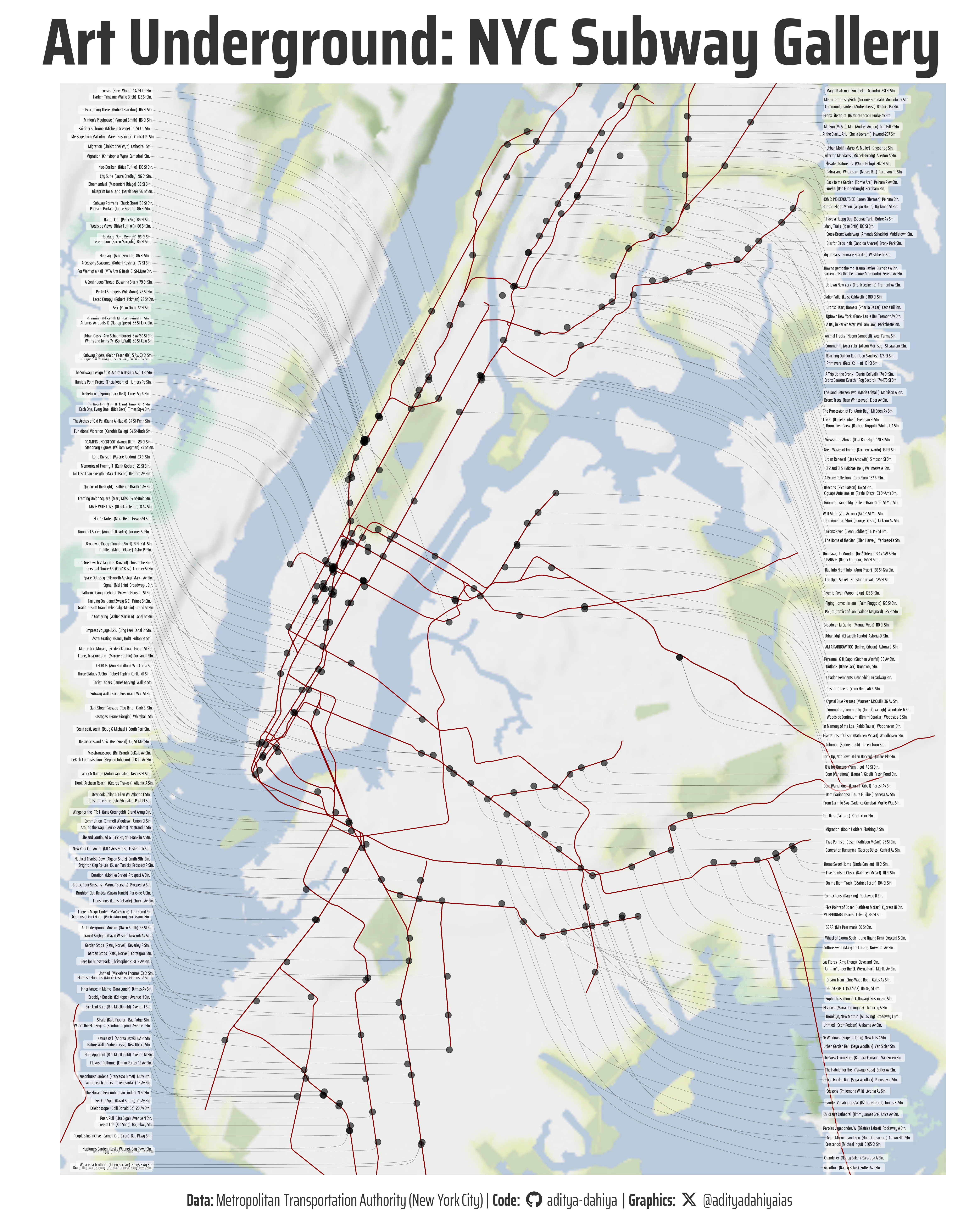
Figure 1: A map of public artworks displayed across Manhattan’s subway stations, showing the Metropolitan Transportation Authority’s permanent art collection. Each label identifies the artwork title, artist, and station location along the transit network.
How the Graphic Was Created
This visualization was built using R’s powerful ecosystem of spatial and visualization packages. The workflow began by geocoding subway station names using tidygeocoder to obtain precise coordinates, then converting the data to spatial format with sf. The base map was created using ggmap with Stadia Maps terrain tiles, processed as raster data through terra. NYC subway line geometries were loaded from a shapefile, spatially cropped to the Manhattan area, and overlaid on the map. The challenging task of labeling multiple artworks without overlap was solved using ggrepel, which intelligently positions labels on opposite sides of the map based on longitude coordinates. Custom nudging variables and curved connection segments ensure clean, readable labels that don’t obscure the underlying geography.
Loading required libraries
Code
pacman::p_load( tidyverse, # All things tidy scales, # Nice Scales for ggplot2 fontawesome, # Icons display in ggplot2 ggtext, # Markdown text support for ggplot2 showtext, # Display fonts in ggplot2 colorspace, # Lighten and Darken colours patchwork # Composing Plots)mta_art <- readr::read_csv('https://raw.githubusercontent.com/rfordatascience/tidytuesday/main/data/2025/2025-07-22/mta_art.csv')station_lines <- readr::read_csv('https://raw.githubusercontent.com/rfordatascience/tidytuesday/main/data/2025/2025-07-22/station_lines.csv')
Visualization Parameters
Code
# Font for titlesfont_add_google("Saira",family ="title_font") # Font for the captionfont_add_google("Saira Condensed",family ="body_font") # Font for plot textfont_add_google("Saira Extra Condensed",family ="caption_font") showtext_auto()# A base Colourbg_col <-"white"seecolor::print_color(bg_col)# Colour for highlighted texttext_hil <-"grey20"seecolor::print_color(text_hil)# Colour for the texttext_col <-"grey20"seecolor::print_color(text_col)line_col <-"grey30"# Define Base Text Sizebts <-120mypal <- paletteer::paletteer_d("fishualize::Balistapus_undulatus")mypal <-c("#DD75D3", "#E16305", "#F2CB05", "#719F4F", "#7E8CFF")# Caption stuff for the plotsysfonts::font_add(family ="Font Awesome 6 Brands",regular = here::here("docs", "Font Awesome 6 Brands-Regular-400.otf"))github <-""github_username <-"aditya-dahiya"xtwitter <-""xtwitter_username <-"@adityadahiyaias"social_caption_1 <- glue::glue("<span style='font-family:\"Font Awesome 6 Brands\";'>{github};</span> <span style='color: {text_hil}'>{github_username} </span>")social_caption_2 <- glue::glue("<span style='font-family:\"Font Awesome 6 Brands\";'>{xtwitter};</span> <span style='color: {text_hil}'>{xtwitter_username}</span>")plot_caption <-paste0("**Data:** Metropolitan Transportation Authority (New York City)", " | **Code:** ", social_caption_1, " | **Graphics:** ", social_caption_2 )rm(github, github_username, xtwitter, xtwitter_username, social_caption_1, social_caption_2)# Add text to plot-------------------------------------------------plot_title <-"Art Underground: NYC Subway Gallery"
Exploratory Data Analysis and Wrangling
Code
pacman::p_load(summarytools)mta_art |>dfSummary() |>view()station_lines |>dfSummary() |>view()pacman::p_load(tidygeocoder)# Try to get geographical locations of the mapsdf1 <- station_lines |>distinct(station_name) |>mutate(station_name =paste0(station_name, " Station, New York City")) |>geocode( station_name, method ='osm', lat = latitude , long = longitude )df2 <- df1 |>drop_na() |>mutate(full_station_name = station_name,station_name =str_remove(station_name, " Station, New York City") ) |>st_as_sf(coords =c("longitude", "latitude"),crs ="EPSG:4326" )df3 <- df2 |>bind_cols(st_coordinates(df2) |> janitor::clean_names() )plotdf <- mta_art |>left_join(df3) |>filter(!is.na(x) &!is.na(y)) |># Remove values outside my map's bounding boxfilter(x <-73.83& x >-74.1) |>filter(y <40.88& y >40.6) |>st_as_sf() |># Add a minor jitter in the positions to prevent overlaps in multiple# artworks within the same subway stationst_jitter(0.001)mid_lon <-mean(plotdf$x, na.rm = T)mid_lat <-mean(plotdf$y, na.rm = T)# Create new directional variables using tidyverseplotdf2 <- plotdf |>select(-agency, -art_image_link, -art_description, art_date, -line) |># Create the directional variablesmutate(# lon_var: east if longitude > mid_lon, west otherwiselon_var =case_when( x > mid_lon ~"east", x <= mid_lon ~"west" ),# lat_var: north if latitude > mid_lat, south otherwiselat_var =case_when( y > mid_lat ~"north", y <= mid_lat ~"south" ),# nudge_x_var to create a variable for nudge x with ggrepelnudge_x_var =if_else( lon_var =="east", -73.82- x,-74.05- x ),segment_curv_var =if_else( lat_var =="north",-0.5,0.5 ) )
Getting New York City Base Map
Code
pacman::p_load(ggmap, tidyterra)# Define your bounding boxmy_bbox <-c(bottom =40.6, top =40.88,left =-74.08, right =-73.78)base_map_rast <-get_stadiamap(bbox = my_bbox,zoom =11,maptype ="stamen_terrain_background") |> terra::rast()ggplot() +geom_spatraster_rgb(data = base_map_rast )
# Saving a thumbnaillibrary(magick)# Saving a thumbnail for the webpageimage_read(here::here("data_vizs", "tidy_mta_art_catalog.png")) |>image_resize(geometry ="x400") |>image_write( here::here("data_vizs", "thumbnails", "tidy_mta_art_catalog.png" ) )
Session Info
Code
pacman::p_load( tidyverse, # All things tidy scales, # Nice Scales for ggplot2 fontawesome, # Icons display in ggplot2 ggtext, # Markdown text support for ggplot2 showtext, # Display fonts in ggplot2 colorspace, # Lighten and Darken colours patchwork # Composing Plots)sessioninfo::session_info()$packages |>as_tibble() |> dplyr::select(package, version = loadedversion, date, source) |> dplyr::arrange(package) |> janitor::clean_names(case ="title" ) |> gt::gt() |> gt::opt_interactive(use_search =TRUE ) |> gtExtras::gt_theme_espn()
Table 1: R Packages and their versions used in the creation of this page and graphics