APOD Archive: Image processing and color analysis

Creating color-sorted image collages using {magick}, {ggplot2}, and {colorspace}

#TidyTuesday

{magick}

Astronomy

Author

Aditya Dahiya

Published

January 23, 2026

About the Data

The Astronomy Picture of the Day (APOD) archive dataset comes from NASA’s popular website that features daily astronomy-related images with scientific explanations. This dataset, curated by Erin Grand and packaged in the {astropic} R package, contains image information spanning from 2007 to 2025. Each entry includes metadata such as the image title, date, explanation, copyright holder, media type (image or video), and URLs for both standard and high-resolution versions when available. The dataset is part of the TidyTuesday project, a weekly data project in the R for Data Science community, and can be accessed through various programming languages including R, Python, and Julia. Participants can explore questions like what types of celestial objects appear most frequently in the archive or whether any images have been featured multiple times, making it an excellent resource for practicing data analysis and visualization skills.

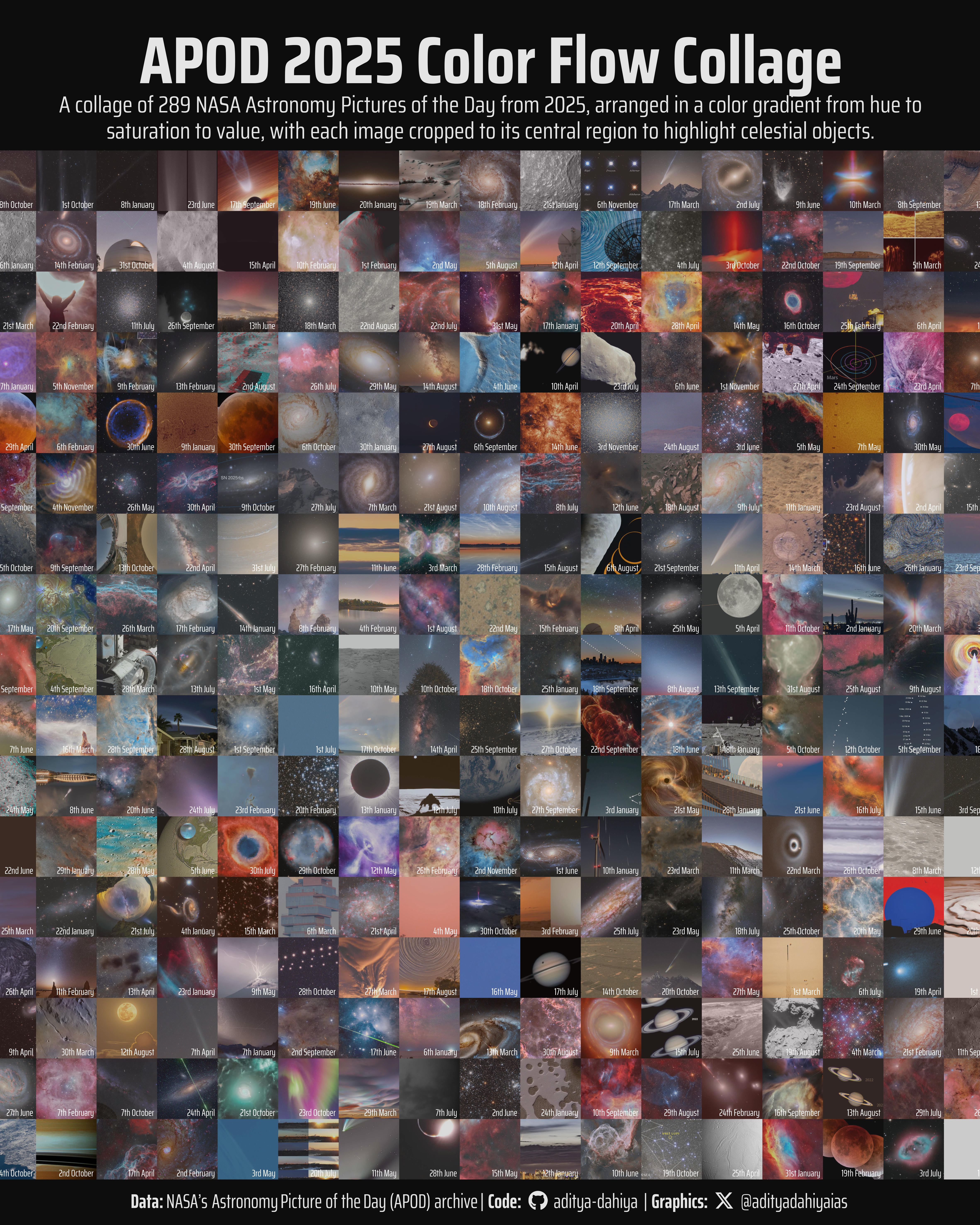
Figure 1: This visualization showcases the stunning diversity of NASA’s Astronomy Picture of the Day archive from 2025. Each image was processed to extract its central 50% area and dominant color, then arranged to create a smooth color gradient from top-left to bottom-right. The semi-transparent overlay reveals the underlying color flow pattern across the astronomical imagery.

How I Made This Graphic

Loading required libraries

Code

pacman::p_load(
  tidyverse, # All things tidy

  scales, # Nice Scales for ggplot2
  fontawesome, # Icons display in ggplot2
  ggtext, # Markdown text support for ggplot2
  showtext, # Display fonts in ggplot2
  colorspace, # Lighten and Darken colours
  sf, # Spatial Features

  patchwork,  # Composing Plots
  packcircles, # for hierarchichal packing circles
  colorspace, # Modify and play with colours, extract dominant colours
  magick  # Playing with images
)

apod <- readr::read_csv('https://raw.githubusercontent.com/rfordatascience/tidytuesday/main/data/2026/2026-01-20/apod.csv')

Visualization Parameters

Code

# Font for titles
font_add_google("Saira",
  family = "title_font"
)

# Font for the caption
font_add_google("Saira Condensed",
  family = "body_font"
)

# Font for plot text
font_add_google("Saira Extra Condensed",
  family = "caption_font"
)

showtext_auto()

# A base Colour
bg_col <- "grey5"
seecolor::print_color(bg_col)

# Colour for highlighted text
text_hil <- "grey90"
seecolor::print_color(text_hil)

# Colour for the text
text_col <- "grey80"
seecolor::print_color(text_col)

# Define Base Text Size
bts <- 120

# Caption stuff for the plot
sysfonts::font_add(
  family = "Font Awesome 6 Brands",
  regular = here::here("docs", "Font Awesome 6 Brands-Regular-400.otf")
)
github <- "&#xf09b"
github_username <- "aditya-dahiya"
xtwitter <- "&#xe61b"
xtwitter_username <- "@adityadahiyaias"
social_caption_1 <- glue::glue("<span style='font-family:\"Font Awesome 6 Brands\";'>{github};</span> <span style='color: {text_hil}'>{github_username}  </span>")
social_caption_2 <- glue::glue("<span style='font-family:\"Font Awesome 6 Brands\";'>{xtwitter};</span> <span style='color: {text_hil}'>{xtwitter_username}</span>")
plot_caption <- paste0(
  "**Data:**  NASA's Astronomy Picture of the Day (APOD) archive",
  " |  **Code:** ",
  social_caption_1,
  " |  **Graphics:** ",
  social_caption_2
)
rm(
  github, github_username, xtwitter,
  xtwitter_username, social_caption_1,
  social_caption_2
)

plot_title <- "APOD 2025 Color Flow Collage"

plot_subtitle <- "A collage of 289 NASA Astronomy Pictures of the Day from 2025, arranged in a color gradient from hue to saturation to value, with each image cropped to its central region to highlight celestial objects." |> 
  str_wrap(110)

Exploratory Data Analysis and Wrangling

Code

bts = 120

# Filtered data
apod_2025 <- apod |> 
  filter(media_type == "image") |> 
  filter(date >= as_date("2025-01-01")) |> 
  select(date, url, title) |> 
  filter(!is.na(url))

# Take only 289 images (17x17 = 289), to get a square number
apod_2025 <- apod_2025 |> slice(1:300)

# Function to extract dominant color from an image
get_dominant_color <- function(img) {
  # Resize to 1x1 to get average color
  img_tiny <- image_scale(img, "1x1!")
  col <- image_data(img_tiny, channels = "rgb")
  rgb(col[1], col[2], col[3], maxColorValue = 255)
}

# Function to process each image with robust error handling
# Extracts central 50% to avoid borders and text
process_image <- function(url, index = NULL) {
  tryCatch({
    if (!is.null(index)) {
      message(sprintf("Processing image %d: %s", index, url))
    }
    
    # Read image with timeout
    img <- image_read(url)
    
    # Get dimensions
    info <- image_info(img)
    
    # Validate image was read successfully
    if (info$width == 0 || info$height == 0) {
      message(paste("Invalid image dimensions for:", url))
      return(NULL)
    }
    
    # Calculate central 50% dimensions
    # This removes 25% from each side
    central_width <- info$width * 0.5
    central_height <- info$height * 0.5
    x_offset <- info$width * 0.25
    y_offset <- info$height * 0.25
    
    # Crop to central 50% area
    img_central <- image_crop(img, 
                              geometry = geometry_area(
                                width = central_width,
                                height = central_height,
                                x_off = x_offset,
                                y_off = y_offset
                              ))
    
    # Get info of cropped image
    central_info <- image_info(img_central)
    
    # Now crop that central area to a square
    min_dim <- min(central_info$width, central_info$height)
    img_square <- image_crop(img_central, 
                             geometry = geometry_area(
                               width = min_dim,
                               height = min_dim,
                               x_off = (central_info$width - min_dim) / 2,
                               y_off = (central_info$height - min_dim) / 2
                             ))
    
    # Resize to 600x600
    img_resized <- image_scale(img_square, "600x600!")
    
    # Extract dominant color
    dominant_color <- get_dominant_color(img_resized)
    
    message(paste("✓ Successfully processed:", url))
    list(image = img_resized, color = dominant_color, url = url)
    
  }, error = function(e) {
    message(paste("✗ Error processing:", url))
    message(paste("  Error message:", e$message))
    return(NULL)
  })
}

# Process all images with progress tracking
processed_images <- map2(
  apod_2025$url, 
  seq_along(apod_2025$url),
  process_image,
  .progress = TRUE
)

# Filter out NULL entries and update dataset
valid_idx <- map_lgl(processed_images, ~!is_null(.x))
n_failed <- sum(!valid_idx)
n_success <- sum(valid_idx)

message(sprintf("\n=== Processing Summary ==="))
message(sprintf("Successfully processed: %d images", n_success))
message(sprintf("Failed to process: %d images", n_failed))
message(sprintf("Success rate: %.1f%%", (n_success/length(valid_idx))*100))

processed_images <- processed_images[valid_idx]
apod_2025_clean <- apod_2025[valid_idx, ]

# If we have fewer than 289 images, adjust grid size
n_images <- length(processed_images)
grid_size <- floor(sqrt(n_images))
n_to_use <- grid_size^2

message(
  sprintf(
    "\nCreating %dx%d grid with %d images", grid_size, grid_size, n_to_use
    )
  )

# Take only the number we need for a perfect square
processed_images <- processed_images[1:n_to_use]
apod_2025_clean <- apod_2025_clean[1:n_to_use, ]

# Continue with the rest of the code...

# Process all images (this will take some time!)
message("Processing images... This may take several minutes.")
# processed_images <- map(apod_2025$url, process_image, .progress = TRUE)

# Remove any NULL entries (failed downloads)
valid_idx <- map_lgl(processed_images, ~!is_null(.x))
processed_images <- processed_images[valid_idx]
apod_2025_clean <- apod_2025_clean[valid_idx, ]

# Extract colors and images
colors <- map_chr(processed_images, ~.x$color)
images <- map(processed_images, ~.x$image)

# Convert colors to HSV for sorting
color_hsv <- t(rgb2hsv(col2rgb(colors)))
apod_2025_clean$hue <- color_hsv[, 1]
apod_2025_clean$saturation <- color_hsv[, 2]
apod_2025_clean$value <- color_hsv[, 3]
apod_2025_clean$color <- colors

# Sort by hue, then saturation, then value for color flow
apod_sorted <- apod_2025_clean |> 
  arrange(hue, saturation, value)

# Reorder images based on sorting
images_sorted <- images[match(apod_sorted$date, apod_2025$date)]

# Create collage
message("Creating collage...")
n_cols <- grid_size
n_rows <- grid_size

# Combine images into rows
rows <- list()
for (i in 1:n_rows) {
  start_idx <- (i - 1) * n_cols + 1
  end_idx <- min(i * n_cols, length(images_sorted))
  
  if (start_idx <= length(images_sorted)) {
    row_images <- images_sorted[start_idx:end_idx]
    rows[[i]] <- image_append(do.call(c, row_images))
  }
}

# Combine rows vertically
collage <- image_append(do.call(c, rows), stack = TRUE)

# Save the collage
message("Saving collage...")
image_write(
  collage, 
  path = here::here(
    "data_vizs",
    "tidy_nasa_astronomy_pics.png"
  ), 
  quality = 95
  )

# Create a ggplot2 visualization showing the color distribution
color_grid <- apod_sorted |> 
  slice(1:(grid_size^2)) |>
  mutate(
    row = rep(1:grid_size, each = grid_size),
    col = rep(1:grid_size, times = grid_size)
  )

library(tidyverse)
library(magick)
library(colorspace)
library(patchwork)  # Optional: for better composition

# First, create the actual collage image using magick
message("Creating collage with magick...")
n_cols <- grid_size  # or 17 if you have exactly 289 images
n_rows <- grid_size

# Combine images into rows
rows <- list()
for (i in 1:n_rows) {
  start_idx <- (i - 1) * n_cols + 1
  end_idx <- min(i * n_cols, length(images_sorted))
  
  if (start_idx <= length(images_sorted)) {
    row_images <- images_sorted[start_idx:end_idx]
    rows[[i]] <- image_append(do.call(c, row_images))
  }
}

# Combine rows vertically
collage <- image_append(do.call(c, rows), stack = TRUE)

image_write(
  collage, 
  path = here::here(
    "data_vizs",
    "tidy_nasa_astronomy_pics.png"
  ),  
  quality = 50
  )

# Read the collage back for ggplot2
collage_for_ggplot <- image_read(
  here::here(
    "data_vizs",
    "tidy_nasa_astronomy_pics.png"
  )
)

# First, prepare the date labels in the desired format
color_grid <- color_grid |> 
  mutate(
    date_label = format(date, "%d") |> 
      as.numeric() |> 
      # Add ordinal suffix (1st, 2nd, 3rd, etc.)
      sapply(function(d) {
        suffix <- case_when(
          d %in% c(11, 12, 13) ~ "th",
          d %% 10 == 1 ~ "st",
          d %% 10 == 2 ~ "nd",
          d %% 10 == 3 ~ "rd",
          TRUE ~ "th"
        )
        paste0(d, suffix)
      }) |> 
      # Combine with month name
      paste(format(date, "%B"))
  )

The Plot

Code

bts = 120

# Create the plot with actual images as background and color overlay
g <- ggplot(
  color_grid, 
  mapping = aes(
    x = col, 
    y = row
  )
) +
  # Add the actual collage as background using annotation_raster
  annotation_raster(
    collage_for_ggplot,
    xmin = 0.5, xmax = n_cols + 0.5,
    ymin = 0.5, ymax = n_rows + 0.5,
    interpolate = TRUE
  ) +
  # Overlay with semi-transparent color tiles
  geom_tile(aes(fill = color), alpha = 0.3, color = NA) +
  # Add date labels in bottom right corner of each tile
  geom_text(
    aes(label = date_label),
    hjust = 1,
    vjust = 0,
    nudge_x = 0.45,   # Position near right edge
    nudge_y = -0.45,  # Position near bottom edge
    family = "caption_font",
    color = "white",
    size = bts / 10,
    fontface = "plain"
  ) +
  scale_fill_identity() +
  scale_x_continuous(expand = c(0, 0), limits = c(0.5, n_cols + 0.5)) +
  scale_y_continuous(expand = c(0, 0), limits = c(0.5, n_rows + 0.5)) +
  coord_fixed() +
  labs(
    title = plot_title,
    subtitle = plot_subtitle,
    x = NULL,
    y = NULL,
    caption = plot_caption
  ) +
  theme_void(
    base_family = "body_font",
    base_size = bts * 3
  ) +
  theme(
    legend.position = "none",
    # Overall
    text = element_text(
      margin = margin(0, 0, 0, 0, "mm"),
      colour = text_hil,
      lineheight = 0.3
    ),
    plot.title = element_text(
      margin = margin(10, 0, 0, 0, "mm"),
      lineheight = 0.3,
      hjust = 0.5,
      size = 2 * bts,
      face = "bold"
    ),
    plot.subtitle = element_text(
      margin = margin(0, 0, 3, 0, "mm"),
      hjust = 0.5,
      size = 0.7 * bts,
      lineheight = 0.3
    ),
    plot.caption = element_textbox(
      margin = margin(5, 0, 0, 0, "mm"),
      hjust = 0.5,
      halign = 0.5,
      family = "caption_font",
      size = bts * 0.6
    ),
    plot.caption.position = "plot",
    plot.title.position = "plot",
    plot.margin = margin(-10, -10, -10, -10, "mm")
  )

# Save the plot
ggsave(
  filename = here::here(
    "data_vizs",
    "tidy_nasa_astronomy_pics_1.png"
  ),
  plot = g,
  width = 400,
  height = 500,
  units = "mm",
  bg = bg_col
)

Savings the thumbnail for the webpage

Code

# Saving a thumbnail

library(magick)

# Saving a thumbnail for the webpage
image_read(
  here::here(
    "data_vizs",
    "tidy_nasa_astronomy_pics_1.png"
    )
  ) |>
  image_resize(geometry = "x400") |>
  image_write(
    here::here(
      "data_vizs",
      "thumbnails",
      "tidy_nasa_astronomy_pics.png"
    )
  )

Session Info

Code

pacman::p_load(
  tidyverse, # All things tidy

  scales, # Nice Scales for ggplot2
  fontawesome, # Icons display in ggplot2
  ggtext, # Markdown text support for ggplot2
  showtext, # Display fonts in ggplot2
  colorspace, # Lighten and Darken colours
  sf, # Spatial Features

  patchwork,  # Composing Plots
  packcircles # for hierarchichal packing circles
)

sessioninfo::session_info()$packages |>
  as_tibble() |>
  
  # The attached column is TRUE for packages that were 
  # explicitly loaded with library()
  dplyr::filter(attached == TRUE) |>
  dplyr::select(package,
    version = loadedversion,
    date, source
  ) |>
  dplyr::arrange(package) |>
  janitor::clean_names(
    case = "title"
  ) |>
  gt::gt() |>
  gt::opt_interactive(
    use_search = TRUE
  ) |>
  gtExtras::gt_theme_espn()

Table 1: R Packages and their versions used in the creation of this page and graphics

About the Data

How I Made This Graphic

Loading required libraries

Visualization Parameters

Exploratory Data Analysis and Wrangling

The Plot

Savings the thumbnail for the webpage

Session Info

Links