Creating ridge-density plots and uncovering viewership patterns in Netflix’s movie catalog.
#TidyTuesday
{ggridges}
Density Ridges Plot
Author
Aditya Dahiya
Published
July 30, 2025
About the Data
This analysis uses Netflix viewing data from the TidyTuesday project (Week 30, 2025), which compiles viewing statistics from Netflix’s official Engagement Reports spanning late 2023 through the first half of 2025. The dataset, curated by Jen Richmond from RLadies-Sydney, captures approximately 99% of all Netflix viewing activity, representing over 95 billion hours of content consumption across a diverse range of genres and languages. The data includes two main components: movies and TV shows, with detailed information on viewing hours, release dates, runtime, global availability status, and calculated view counts (derived from hours viewed divided by runtime). This comprehensive dataset provides insights into viewing patterns, content performance over time, and the relationship between release timing and audience engagement on the world’s leading streaming platform.
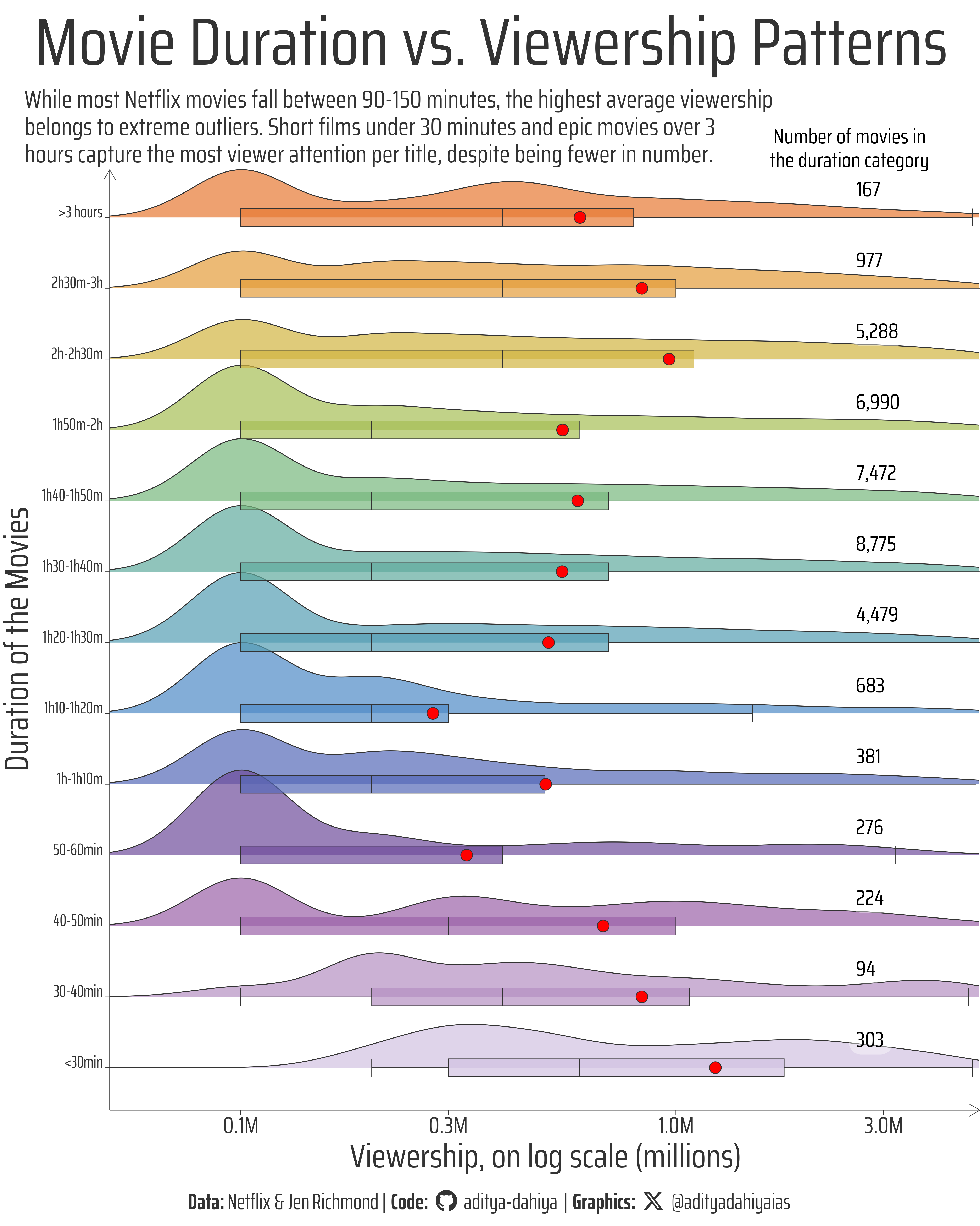
Figure 1: This visualization displays the distribution of Netflix movie viewership across 13 runtime categories, from under 30 minutes to over 3 hours. Each row shows a density ridge plot revealing the spread of viewership within that duration category, overlaid with boxplots indicating quartiles and outliers. Red dots mark the trimmed mean viewership for each category, while numbers on the right show the count of movies in each runtime bin. The x-axis uses a logarithmic scale to accommodate the wide range of viewership values.
How the Graphic Was Created
This visualization was created using R and the tidyverse ecosystem, combining multiple layers to reveal Netflix movie viewership patterns across runtime categories. I first converted the runtime strings (e.g., “1H 30M 0S”) into numerical hours using lubridate’sduration() function and custom regex extraction. The movies were then binned into 13 ordered runtime categories using cut() with carefully defined breaks from <30 minutes to >3 hours. The core visualization layers three complementary geoms: geom_density_ridges() from the ggridges package to show the distribution shape of viewership within each runtime category, geom_boxplot() to display statistical summaries (quartiles and outliers), and geom_point() to highlight the trimmed mean viewership for each category. The color palette was sourced from paletteer using the “khroma::smoothrainbow” scheme, while text formatting utilized Google Fonts via showtext and ggtext for enhanced typography. The x-axis employs a log10 transformation with scales formatting to handle the wide range of viewership values, and custom annotations display the count of movies in each duration category to provide context for the distributions.
Loading required libraries
Code
pacman::p_load( tidyverse, # All things tidy scales, # Nice Scales for ggplot2 fontawesome, # Icons display in ggplot2 ggtext, # Markdown text support for ggplot2 showtext, # Display fonts in ggplot2 colorspace, # Lighten and Darken colours patchwork, # Composing Plots ggridges, # Making ridgeline plot gghalves # Half geoms in ggplot2)movies <- readr::read_csv('https://raw.githubusercontent.com/rfordatascience/tidytuesday/main/data/2025/2025-07-29/movies.csv')shows <- readr::read_csv('https://raw.githubusercontent.com/rfordatascience/tidytuesday/main/data/2025/2025-07-29/shows.csv')
Visualization Parameters
Code
# Font for titlesfont_add_google("Saira",family ="title_font") # Font for the captionfont_add_google("Saira Condensed",family ="body_font") # Font for plot textfont_add_google("Saira Extra Condensed",family ="caption_font") showtext_auto()# A base Colourbg_col <-"white"seecolor::print_color(bg_col)# Colour for highlighted texttext_hil <-"grey20"seecolor::print_color(text_hil)# Colour for the texttext_col <-"grey20"seecolor::print_color(text_col)line_col <-"grey30"# Define Base Text Sizebts <-80# Caption stuff for the plotsysfonts::font_add(family ="Font Awesome 6 Brands",regular = here::here("docs", "Font Awesome 6 Brands-Regular-400.otf"))github <-""github_username <-"aditya-dahiya"xtwitter <-""xtwitter_username <-"@adityadahiyaias"social_caption_1 <- glue::glue("<span style='font-family:\"Font Awesome 6 Brands\";'>{github};</span> <span style='color: {text_hil}'>{github_username} </span>")social_caption_2 <- glue::glue("<span style='font-family:\"Font Awesome 6 Brands\";'>{xtwitter};</span> <span style='color: {text_hil}'>{xtwitter_username}</span>")plot_caption <-paste0("**Data:** Netflix & Jen Richmond", " | **Code:** ", social_caption_1, " | **Graphics:** ", social_caption_2 )rm(github, github_username, xtwitter, xtwitter_username, social_caption_1, social_caption_2)# Add text to plot-------------------------------------------------plot_title <-"Movie Duration vs. Viewership Patterns"plot_subtitle <-"While most Netflix movies fall between 90-150 minutes, the highest average viewership belongs to extreme outliers. Short films under 30 minutes and epic movies over 3 hours capture the most viewer attention per title, despite being fewer in number."|>str_wrap(85)str_view(plot_subtitle)
Exploratory Data Analysis and Wrangling
Code
# Credits: Claude Sonnet 4.0# Function to convert runtime string to durationconvert_runtime <-function(runtime_string) {# Extract hours, minutes, and seconds using regex hours <-str_extract(runtime_string, "\\d+(?=H)") |>as.numeric() minutes <-str_extract(runtime_string, "\\d+(?=M)") |>as.numeric() seconds <-str_extract(runtime_string, "\\d+(?=S)") |>as.numeric()# Replace NA with 0 hours <-ifelse(is.na(hours), 0, hours) minutes <-ifelse(is.na(minutes), 0, minutes) seconds <-ifelse(is.na(seconds), 0, seconds)# Create duration objectduration(hours = hours, minutes = minutes, seconds = seconds)}# Apply to movies dataframemovies <- movies |>mutate(# Convert duration to a numerical / time duration variableruntime_duration =convert_runtime(runtime),# Convert runtime to hours for better visualizationruntime_hours =as.numeric(runtime_duration, "hours") )# Apply to shows dataframeshows <- shows |>mutate(# Convert duration to a numerical / time duration variableruntime_duration =convert_runtime(runtime),# Convert runtime to hours for better visualizationruntime_hours =as.numeric(runtime_duration, "hours") )# Explore the data with summarytools# pacman::p_load(summarytools)# movies |> # dfSummary() |> # view()# # # shows |> # dfSummary() |> # view()# Some trial examples to detect pattern in shows and movies duration# shows |> # ggplot(# mapping = aes(# x = as.numeric(runtime_duration, "hours")# )# ) +# geom_boxplot(alpha = 0.2) +# scale_x_log10(name = "Runtime (hours)")# # shows |> # ggplot(# mapping = aes(# x = as.numeric(runtime_duration, "hours"),# y = hours_viewed# )# ) +# geom_point(# alpha = 0.3# ) +# geom_smooth() +# scale_x_log10(name = "Runtime (hours)")# # # shows |> # ggplot(# mapping = aes(# x = as.numeric(runtime_duration, "hours"),# y = hours_viewed# )# ) +# geom_violin() +# scale_x_log10(name = "Runtime (hours)")# # # I took some Ideas from AI: Claude Sonnet 4.0# library(ggridges) # For ridge plots# # movies |> # select(runtime_hours, hours_viewed, views) |> # filter(runtime_hours > (1/2) & runtime_hours < 3) |> # ggplot(aes(runtime_hours)) +# geom_boxplot()# Planning a RIDGE PLOT - Shows distribution of views across runtime binsdf1 <- movies |>select(runtime_hours, hours_viewed, views) |>mutate(runtime_bin =cut( runtime_hours, breaks =c(0, 0.5, 0.67, 0.83, 1, 1.17, 1.33, 1.5, 1.67, 1.83, 2, 2.5, 3, Inf),labels =c("<30min", "30-40min", "40-50min", "50-60min", "1h-1h10m", "1h10-1h20m", "1h20-1h30m", "1h30-1h40m", "1h40-1h50m", "1h50m-2h", "2h-2h30m", "2h30m-3h", ">3 hours" ),include.lowest =TRUE,ordered_result =TRUE ) ) |>filter(!is.na(runtime_bin),!is.na(views),is.finite(views), views >0, # Remove zero or negative views views <Inf# Remove infinite values )# df1$runtime_bin |> levels()# pacman::p_load(ggridges, gghalves)# df1 |> # count(runtime_bin)df2 <- df1 |>group_by(runtime_bin) |>summarise(mean_views =mean(views, na.rm = T, trim =0.1),median_views =median(views, na.rm = T) )
# Saving a thumbnaillibrary(magick)# Saving a thumbnail for the webpageimage_read(here::here("data_vizs", "tidy_netflix_data.png")) |>image_resize(geometry ="x400") |>image_write( here::here("data_vizs", "thumbnails", "tidy_netflix_data.png" ) )
Session Info
Code
pacman::p_load( tidyverse, # All things tidy scales, # Nice Scales for ggplot2 fontawesome, # Icons display in ggplot2 ggtext, # Markdown text support for ggplot2 showtext, # Display fonts in ggplot2 colorspace, # Lighten and Darken colours patchwork # Composing Plots)sessioninfo::session_info()$packages |>as_tibble() |> dplyr::select(package, version = loadedversion, date, source) |> dplyr::arrange(package) |> janitor::clean_names(case ="title" ) |> gt::gt() |> gt::opt_interactive(use_search =TRUE ) |> gtExtras::gt_theme_espn()
Table 1: R Packages and their versions used in the creation of this page and graphics