Palm Trees’ Species: Skyward or Sprawling

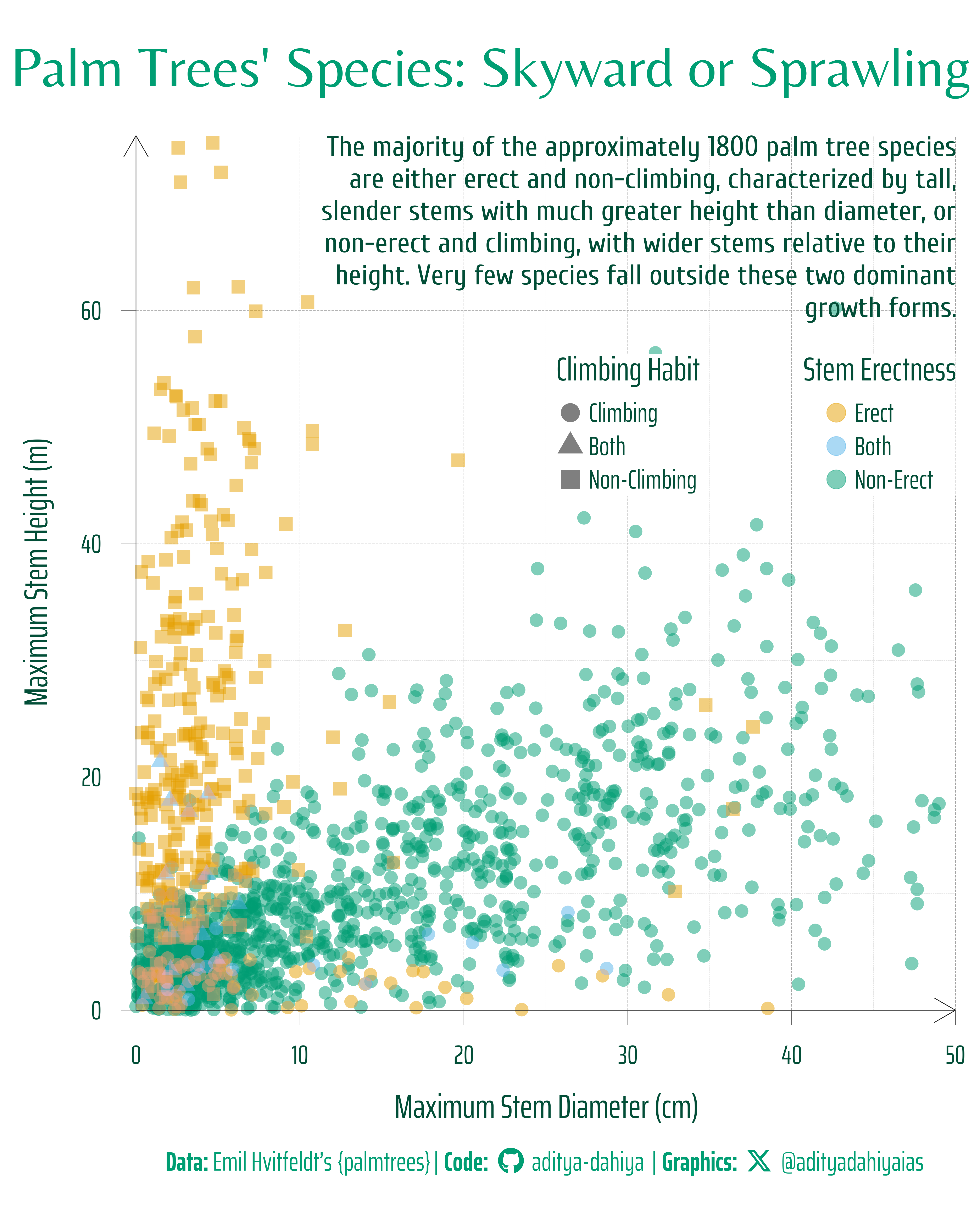
The majority of the approximately 1800 palm tree species are either erect and non-climbing, characterized by tall, slender stems with much greater height than diameter, or non-erect and climbing, with wider stems relative to their height. Very few species fall outside these two dominant growth forms.

About the Data

The dataset for this week’s exploration of Palm Trees is sourced from the PalmTraits 1.0 database, a comprehensive global compilation of functional traits for palms (Arecaceae), a plant family pivotal in tropical and subtropical ecosystems. Accessible via the palmtrees R package developed by Emil Hvitfeldt, this dataset was curated by Lydia Gibson for TidyTuesday. It includes detailed taxonomic information such as species names (spec_name), genus (acc_genus), and subfamily (palm_subfamily), alongside functional traits like growth habits (e.g., climbing, acaulescent, erect), stem characteristics (e.g., max_stem_height_m, stem_armed), leaf dimensions (e.g., max__blade__length_m), and fruit properties (e.g., average_fruit_length_cm, main_fruit_colors).

Figure 1: A scatterplot showing maximum stem diameter (cm) on the X-axis and maximum stem diameter (m) on the Y-axis. The colours of dots refer to the stem-erectness and shape of dots refer to climbing habit. An important technique is the use of blending of colours using {ggblend} to ensure that near the origin of the graph, the overlapping points don’t lead to a loss of visual pattern. The two groups of palm trees’ species emerge which is distinctly visible.

How I made this graphic?

Loading required libraries

# Data Import and Wrangling Tools
library(tidyverse)            # All things tidy

# Final plot tools
library(scales)               # Nice Scales for ggplot2
library(fontawesome)          # Icons display in ggplot2
library(ggtext)               # Markdown text support for ggplot2
library(showtext)             # Display fonts in ggplot2
library(colorspace)           # Lighten and Darken colours

palmtrees <- readr::read_csv('https://raw.githubusercontent.com/rfordatascience/tidytuesday/main/data/2025/2025-03-18/palmtrees.csv')

Visualization Parameters

# Font for titles
font_add_google("Belleza",
  family = "title_font"
) 

# Font for the caption
font_add_google("Saira Extra Condensed",
  family = "caption_font"
) 

# Font for plot text
font_add_google("Cuprum",
  family = "body_font"
) 

showtext_auto()

mypal <- paletteer::paletteer_d("ltc::trio3")
# cols4all::c4a_gui()

# A base Colour
bg_col <- "white"
seecolor::print_color(bg_col)

# Colour for highlighted text
text_hil <- mypal[3]
seecolor::print_color(text_hil)

# Colour for the text
text_col <- colorspace::darken("#009E73", 0.5)
seecolor::print_color(text_col)

line_col <- "grey30"

# Define Base Text Size
bts <- 120

# Caption stuff for the plot
sysfonts::font_add(
  family = "Font Awesome 6 Brands",
  regular = here::here("docs", "Font Awesome 6 Brands-Regular-400.otf")
)
github <- "&#xf09b"
github_username <- "aditya-dahiya"
xtwitter <- "&#xe61b"
xtwitter_username <- "@adityadahiyaias"
social_caption_1 <- glue::glue("<span style='font-family:\"Font Awesome 6 Brands\";'>{github};</span> <span style='color: {text_hil}'>{github_username}  </span>")
social_caption_2 <- glue::glue("<span style='font-family:\"Font Awesome 6 Brands\";'>{xtwitter};</span> <span style='color: {text_hil}'>{xtwitter_username}</span>")
plot_caption <- paste0(
  "**Data:** Emil Hvitfeldt's {palmtrees}", 
  " |  **Code:** ", 
  social_caption_1, 
  " |  **Graphics:** ", 
  social_caption_2
  )
rm(github, github_username, xtwitter, 
   xtwitter_username, social_caption_1, 
   social_caption_2)

# Add text to plot-------------------------------------------------
plot_title <- "Palm Trees' Species: Skyward or Sprawling"

plot_subtitle <- "The majority of the approximately 1800 palm tree species are either erect and non-climbing, characterized by tall, slender stems with much greater height than diameter, or non-erect and climbing, with wider stems relative to their height. Very few species fall outside these two dominant growth forms."

# str_view(plot_subtitle)

Exploratory Data Analysis and Wrangling

# 
# psych::describe(palmtrees) |> 
#   gt::gt()
# 
# DataExplorer::create_report(palmtrees)
# 
# palmtrees |> 
#   janitor::tabyl(spec_name)
# 
# palmtrees |> names()
#   
# palmtrees |> 
#   visdat::vis_miss()
# 
# palmtrees |> 
#   select(-fruit_color_description) |> 
#   dfSummary() |> 
#   view()
# 
# palmtrees |> 
#   ggplot(
#     aes(
#       x = average_fruit_length_cm,
#       y = average_fruit_width_cm,
#       colour = fruit_shape
#     )
#   ) +
#   geom_point(alpha = 1) +
#   coord_cartesian(xlim = c(0, 5), ylim = c(0, 5))
#   
# 
# palmtrees |> 
#   select(spec_name,
#          acc_genus,
#          acc_species,
#          max_stem_dia_cm,
#          max_stem_height_m,
#          stem_solitary,
#          climbing) |> 
#   visdat::vis_miss()
# 
# palmtrees |> 
#   select(spec_name,
#          acc_genus,
#          acc_species,
#          max_stem_dia_cm,
#          max_stem_height_m,
#          stem_solitary,
#          climbing, 
#          erect) |> 
#   drop_na() |> 
#   ggplot(
#     mapping = aes(
#       x = max_stem_dia_cm,
#       y = max_stem_height_m,
#       colour = erect,
#       shape = climbing
#     )
#   ) +
#   geom_point(
#     position = position_jitter(
#       width = 3,
#       height = 4
#     ),
#     alpha = 0.5
#   ) +
#   paletteer::scale_colour_paletteer_d("ltc::trio3") +
#   scale_x_continuous(
#     limits = c(0, 50),
#     oob = scales::squish,
#     expand = expansion(0)
#   ) +
#   scale_y_continuous(
#     limits = c(0, 75),
#     oob = scales::squish,
#     expand = expansion(0)
#   ) +
#   coord_equal(
#     clip = "off"
#   ) +
#   theme_classic()

df <- palmtrees |> 
  select(spec_name,
         acc_genus,
         acc_species,
         max_stem_dia_cm,
         max_stem_height_m,
         stem_solitary,
         climbing, 
         erect) |> 
  drop_na() |>   
  mutate(
    climbing = str_to_title(climbing),
    climbing = fct(climbing,
                   levels = c(
                     "Climbing",
                     "Both",
                     "Non-Climbing"
                   )),
    erect = str_to_title(erect),
    erect = fct(erect,
                levels = c(
                  "Erect",
                  "Both",
                  "Non-Erect"
                ))
  )

The Base Plots

Using {ggblend} (Kay 2023) to blend and compose colours

g <- df |> 
  ggplot(
    mapping = aes(
      x = max_stem_dia_cm,
      y = max_stem_height_m,
      colour = erect,
      shape = climbing
    )
  ) +
  geom_point(
    size = 7,
    position = position_jitter(
      width = 3,
      height = 4
    ),
    alpha = 0.5
  ) |> ggblend::blend("lighten") +
  annotate(
    geom = "text",
    colour = text_col,
    x = 50, y = 75,
    hjust = 1,
    vjust = 1,
    size = bts / 3.3,
    label = str_wrap(plot_subtitle, 60),
    lineheight = 0.3,
    family = "body_font"
  ) +
  paletteer::scale_colour_paletteer_d("ltc::trio3") +
  scale_x_continuous(
    limits = c(0, 50),
    # oob = scales::squish,
    expand = expansion(0)
  ) +
  scale_y_continuous(
    limits = c(0, 75),
    # oob = scales::squish,
    expand = expansion(0)
  ) +
  coord_cartesian(
    clip = "off"
  ) +
  guides(
    colour = guide_legend(
      override.aes = list(
        size = 10
      )
    ),
    shape = guide_legend(
      override.aes = list(
        size = 10
      )
    )
  ) +
  labs(
    x = "Maximum Stem Diameter (cm)",
    y = "Maximum Stem Height (m)",
    title = plot_title,
    caption = plot_caption,
    colour = "Stem Erectness",
    shape = "Climbing Habit"
  ) +
  
  theme_classic(
    base_family = "caption_font",
    base_size = bts
  ) +
  theme(
    
    # Overall
    plot.margin = margin(15,10,15,10, "mm"),
    plot.title.position = "plot",
    panel.grid.major = element_line(
      linetype = "longdash",
      linewidth = 0.2,
      colour = "grey60"
    ),
    panel.grid.minor = element_line(
      linetype = "longdash",
      linewidth = 0.1,
      colour = "grey80"
    ),
    
    # Axis Lines
    axis.ticks = element_line(
      colour = line_col,
      linewidth = 0.2
    ),
    axis.line = element_line(
      colour = "grey10",
      arrow = arrow(
        length = unit(10, "mm")
      ),
      linewidth = 0.4
    ),
    axis.ticks.length = unit(6, "mm"),
    text = element_text(
      colour = text_col,
      lineheight = 0.3
    ),
    
    # Axis Text
    axis.text = element_text(
      margin = margin(0,0,0,0, "mm"),
      colour = text_col
    ),
    axis.title = element_text(
      margin = margin(0,0,0,0, "mm"),
      colour = text_col
    ),
    
    # Labels and Strip Text
    plot.title = element_text(
      colour = text_hil,
      margin = margin(5,0,15,0, "mm"),
      size = bts * 1.7,
      lineheight = 0.3,
      hjust = 0.5,
      family = "title_font"
    ),
    plot.caption = element_textbox(
      family = "caption_font",
      margin = margin(10,0,5,0, "mm"),
      hjust = 0.5,
      colour = text_hil
    ),
    
    # Legend
    legend.position = "inside",
    legend.position.inside = c(1, 0.75),
    legend.direction = "vertical",
    legend.box = "horizontal",
    legend.justification.inside = c(1, 1),
    legend.box.margin = margin(0,0,0,0, "mm"),
    legend.margin = margin(0,0,0,0, "mm"),
    legend.title = element_text(
      margin = margin(0,0,5,0, "mm"),
      hjust = 0.5
    ),
    legend.text = element_text(
      margin = margin(2,0,2,3, "mm")
    ),
    legend.title.position = "top"
  )


ggsave(
  filename = here::here(
    "data_vizs",
    "tidy_palm_trees.png"
  ),
  plot = g,
  width = 400,
  height = 500,
  units = "mm",
  bg = bg_col
)

Savings the thumbnail for the webpage

# Saving a thumbnail

library(magick)

# Saving a thumbnail for the webpage
image_read(here::here("data_vizs", 
                      "tidy_palm_trees.png")) |> 
  image_resize(geometry = "x400") |> 
  image_write(
    here::here(
      "data_vizs", 
      "thumbnails", 
      "tidy_palm_trees.png"
    )
  )

Session Info

# Data Import and Wrangling Tools
library(tidyverse)            # All things tidy

# Final plot tools
library(scales)               # Nice Scales for ggplot2
library(fontawesome)          # Icons display in ggplot2
library(ggtext)               # Markdown text support for ggplot2
library(showtext)             # Display fonts in ggplot2
library(colorspace)           # Lighten and Darken colours


sessioninfo::session_info()$packages |> 
  as_tibble() |> 
  select(package, 
         version = loadedversion, 
         date, source) |> 
  arrange(package) |> 
  janitor::clean_names(
    case = "title"
  ) |> 
  gt::gt() |> 
  gt::opt_interactive(
    use_search = TRUE
  ) |> 
  gtExtras::gt_theme_espn()

Table 1: R Packages and their versions used in the creation of this page and graphics

References

Kay, Matthew. 2023. “Ggblend: Blending and Compositing Algebra for ’Ggplot2’.” https://CRAN.R-project.org/package=ggblend.