Plotting Penguins: Bill Dimensions Across Species

This visualization combines the power of ggforce for drawing ellipses and smooth geometry with magick for image annotation and layout. Together, they enhance a standard ggplot2 chart to create a polished, publication-ready graphic using the palmerpenguins dataset.

About the Data

The penguins dataset is included in base R starting from version 4.5.0, and is available via the datasets package. It provides measurements of adult penguins across three species—Adélie, Chinstrap, and Gentoo—found on three islands in the Palmer Archipelago, Antarctica. Key variables include flipper length, body mass, bill dimensions, sex, and the year of observation. This dataset is a curated subset of a more extensive penguins_raw dataset, which also contains information on nesting behavior and blood isotope ratios. Originally used by Gorman et al. (2014) to explore sexual dimorphism in penguins, the dataset gained broader popularity through the palmerpenguins package as a user-friendly alternative to the classic iris dataset. Recent efforts by Kaye et al. (2025) have integrated this data directly into base R, along with reproducible scripts and documentation.

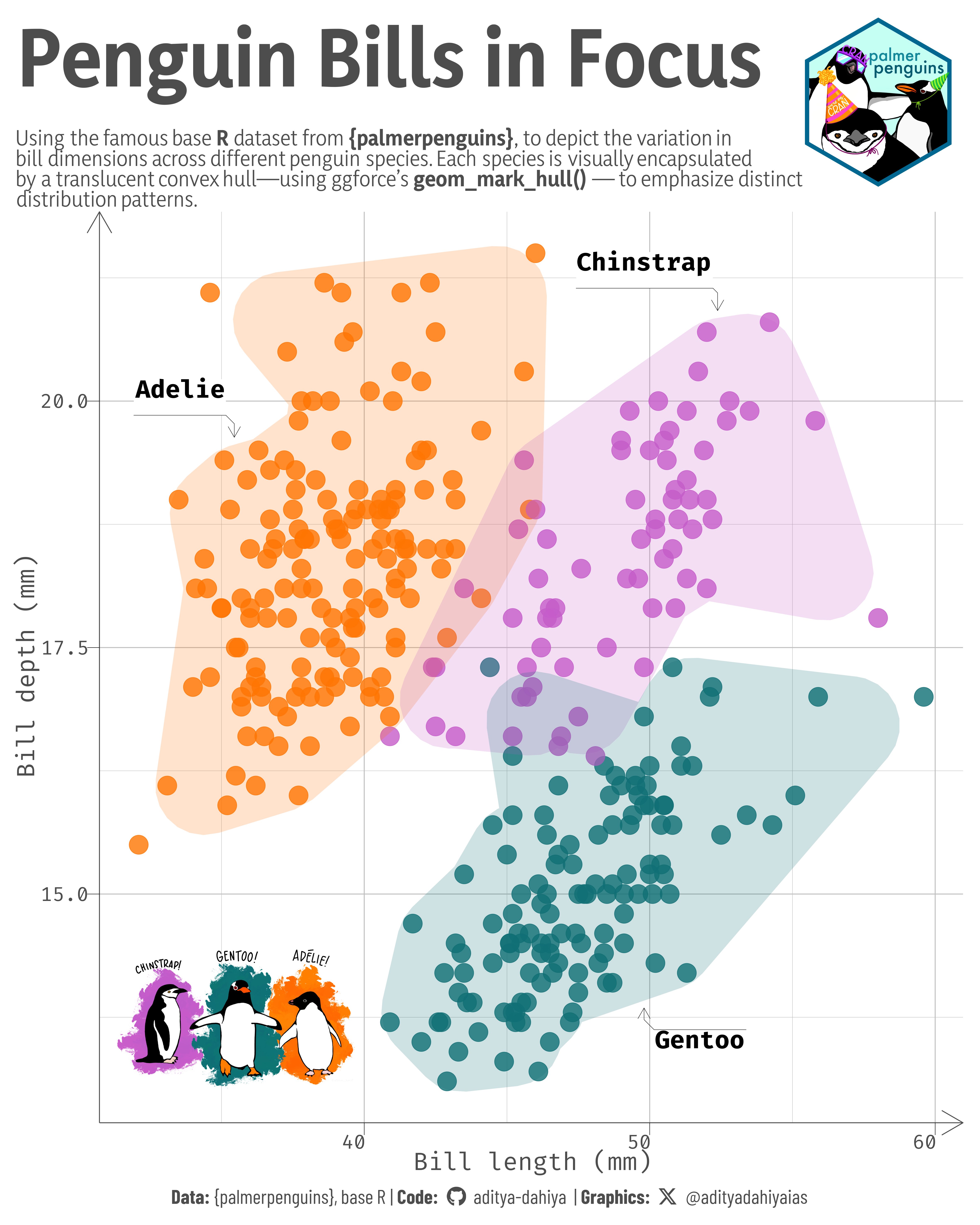
Figure 1: This graphic visualizes the variation in **bill length and depth** across three penguin species—Adélie, Chinstrap, and Gentoo—found in the Palmer Archipelago, Antarctica. Each point represents an individual penguin, with species distinguished by color. Translucent convex hulls, generated using `geom_mark_hull()` from the ggforce package, visually group individuals by species to highlight distinct morphological clusters. The visualization draws from the newly integrated penguins dataset in base R (v4.5.0), offering a clean and engaging way to explore species-level differences in bill dimensions. Penguin illustrations and minimalist typography enhance clarity while maintaining a playful yet informative tone.

How I made this graphic?

To create this visual, I began by loading the penguins dataset now available in base R from version 4.5.0 onwards. Using the tidyverse for data wrangling and ggplot2 for plotting, I mapped bill length and depth, with points styled by species using geom_point(). To highlight species clusters, I used geom_mark_hull() from the ggforce package, which draws translucent convex hulls around each species group. I customized fonts via showtext and google fonts, and embedded penguin illustrations using magick and ggimage. Final layout adjustments, such as adding a logo inset, were done using the patchwork package. The entire plot was saved with ggsave() from [ggplot2] and customized for visual clarity with theme_minimal() and extensive use of element_textbox() from ggtext.

Loading required libraries

# Data Import and Wrangling Tools
library(tidyverse)            # All things tidy

# Final plot tools
library(scales)               # Nice Scales for ggplot2
library(fontawesome)          # Icons display in ggplot2
library(ggtext)               # Markdown text support for ggplot2
library(showtext)             # Display fonts in ggplot2
library(colorspace)           # Lighten and Darken colours

library(magick)               # Download images and edit them
library(ggimage)              # Display images in ggplot2
library(patchwork)            # Composing Plots

library(ggforce)              # for geom_mark_hull()


penguins <- penguins |> 
  as_tibble()

Visualization Parameters

# Font for titles
font_add_google("Yaldevi",
  family = "title_font"
) 

# Font for the caption
font_add_google("Barlow Condensed",
  family = "caption_font"
) 

# Font for plot text
font_add_google("Fira Code",
  family = "body_font"
) 

showtext_auto()

# cols4all::c4a_gui()
# Pick a colour paletter that is Colour-Blind friendly, fair and 
# has a good contrast ratio with white
mypal <- paletteer::paletteer_d("ltc::trio3")

mypal <- c("#FF7502", "#C55CC9", "#0F6F74")

# A base Colour
bg_col <- "white"
seecolor::print_color(bg_col)

# Colour for highlighted text
text_hil <- "grey30"
seecolor::print_color(text_hil)

# Colour for the text
text_col <- "grey30"
seecolor::print_color(text_col)

line_col <- "grey30"

# Define Base Text Size
bts <- 90

# Caption stuff for the plot
sysfonts::font_add(
  family = "Font Awesome 6 Brands",
  regular = here::here("docs", "Font Awesome 6 Brands-Regular-400.otf")
)
github <- "&#xf09b"
github_username <- "aditya-dahiya"
xtwitter <- "&#xe61b"
xtwitter_username <- "@adityadahiyaias"
social_caption_1 <- glue::glue("<span style='font-family:\"Font Awesome 6 Brands\";'>{github};</span> <span style='color: {text_hil}'>{github_username}  </span>")
social_caption_2 <- glue::glue("<span style='font-family:\"Font Awesome 6 Brands\";'>{xtwitter};</span> <span style='color: {text_hil}'>{xtwitter_username}</span>")
plot_caption <- paste0(
  "**Data:** {palmerpenguins}, base R", 
  " |  **Code:** ", 
  social_caption_1, 
  " |  **Graphics:** ", 
  social_caption_2
  )
rm(github, github_username, xtwitter, 
   xtwitter_username, social_caption_1, 
   social_caption_2)

# Add text to plot-------------------------------------------------
plot_title <- "Penguin Bills in Focus"

plot_subtitle <- "Using the famous base **R** dataset from **{palmerpenguins}**, to depict the variation in bill dimensions across different penguin species. Each species is visually encapsulated by a translucent convex hull—using ggforce's **geom_mark_hull()** — to emphasize distinct distribution patterns." |> 
  str_wrap(90) |> 
  str_replace_all("\\n", "<br>")

Exploratory Data Analysis and Wrangling

# library(summarytools)
# penguins |> 
#   dfSummary() |> 
#   view()

# Get images to insert

library(magick)

logo1 <- image_read("https://allisonhorst.github.io/palmerpenguins/reference/figures/lter_penguins.png") |> 
  image_background("transparent")

logo2 <- image_read("https://education.rstudio.com/blog/2020/07/palmerpenguins-cran/penguins_cran.png")

The Plot

g_base <- penguins |> 
  ggplot(
    mapping = aes(
      x = bill_len,
      y = bill_dep
    )
  ) +
  geom_point(
    mapping = aes(
      fill = species,
      colour = species
    ),
    size = 10, 
    alpha = 0.8,
    pch = 21
  ) +
  ggforce::geom_mark_hull(
    mapping = aes(
      fill = species,
      label = species
    ),
    alpha = 0.2,
    colour = "transparent",
    
    expand = unit(5, "mm"),
    radius = unit(20, "mm"),
    concavity = 3,
    
    con.size = 0.2,
    con.type = "elbow",
    con.arrow = arrow(length = unit(5, "mm")),
    show.legend = FALSE,
    label.fontsize = bts,
    label.family = "body_font",
    label.margin = margin(0.5, 0.5, 0.5, 0.5, "mm")
  ) +
  
  # Add a penguins photo
  annotation_custom(
    grid::rasterGrob(logo1),
    xmin = 31, xmax = 40, 
    ymin = 12.5, ymax = 15
  ) +
  scale_colour_manual(
    values = mypal
  ) +
  scale_fill_manual(
    values = mypal
  ) +
  labs(
    title = plot_title,
    subtitle = str_wrap(plot_subtitle, 70),
    caption = plot_caption,
    fill = NULL,
    x = "Bill length (mm)",
    y = "Bill depth (mm)"
  ) +
  theme_minimal(
    base_family = "body_font",
    base_size = bts
  ) +
  theme(
    
    # Overall
    plot.margin = margin(5,5,5,5, "mm"),
    legend.position = "none",
    plot.title.position = "plot",
    text = element_text(
      colour = text_col,
      lineheight = 0.3,
      hjust = 0.5
    ),
    
    # Labels and Strip Text
    plot.title = element_text(
      colour = text_hil,
      margin = margin(5,0,5,0, "mm"),
      size = bts * 3,
      lineheight = 0.3,
      hjust = 0,
      family = "title_font",
      face = "bold"
    ),
    plot.subtitle = element_textbox(
      colour = text_hil,
      margin = margin(5,0,0,0, "mm"),
      size = 0.8 * bts,
      lineheight = 0.3,
      hjust = 0,
      halign = 0,
      family = "title_font"
    ),
    plot.caption = element_textbox(
      margin = margin(5,0,0,0, "mm"),
      hjust = 0.5,
      colour = text_hil,
      size = 0.8 * bts,
      family = "caption_font"
    ),
    plot.caption.position = "plot",
    
    # Axes
    axis.line = element_line(
      colour = text_col,
      arrow = arrow(length = unit(10, "mm")),
      linewidth = 0.5
    ),
    axis.ticks = element_line(linewidth = 0.25),
    axis.ticks.length = unit(5, "mm"),
    axis.title.x = element_text(
      margin = margin(0,0,0,0, "mm")
    ),
    axis.title.y = element_text(
      margin = margin(0,0,0,0, "mm")
    ),
    axis.text.x = element_text(
      margin = margin(0,0,0,0, "mm"),
      hjust = 1
    ),
    axis.text.y = element_text(
      margin = margin(0,0,0,0, "mm"),
      hjust = 1
    ),
    
    # Panel Grid
    panel.grid.major = element_line(
      linewidth = 0.5,
      colour = "grey"
    ),
    panel.grid.minor = element_line(
      linewidth = 0.2,
      colour = "grey"
    )
  )

g_inset <- ggplot() +
  # Add a penguins photo
  annotation_custom(
    grid::rasterGrob(logo2),
    xmin = -Inf, xmax = Inf, 
    ymin = -Inf, ymax = Inf
  ) +
  theme_void()

g <- g_base +
  inset_element(
    p = g_inset,
    left = 0.8, right = 1,
    bottom = 0.85, top = 0.99,
    align_to = "full",
    clip = FALSE
  )
ggsave(
  filename = here::here(
    "data_vizs",
    "tidy_palmerpenguins.png"
  ),
  plot = g,
  width = 400,
  height = 500,
  units = "mm",
  bg = bg_col
)

Savings the thumbnail for the webpage

# Saving a thumbnail

library(magick)

# Saving a thumbnail for the webpage
image_read(here::here("data_vizs", 
                      "tidy_palmerpenguins.png")) |> 
  image_resize(geometry = "x400") |> 
  image_write(
    here::here(
      "data_vizs", 
      "thumbnails", 
      "tidy_palmerpenguins.png"
    )
  )

Session Info

# Data Import and Wrangling Tools
library(tidyverse)            # All things tidy

# Final plot tools
library(scales)               # Nice Scales for ggplot2
library(fontawesome)          # Icons display in ggplot2
library(ggtext)               # Markdown text support for ggplot2
library(showtext)             # Display fonts in ggplot2
library(colorspace)           # Lighten and Darken colours

library(magick)               # Download images and edit them
library(ggimage)              # Display images in ggplot2
library(patchwork)            # Composing Plots

library(ggforce)              # for geom_mark_hull()

sessioninfo::session_info()$packages |> 
  as_tibble() |> 
  select(package, 
         version = loadedversion, 
         date, source) |> 
  arrange(package) |> 
  janitor::clean_names(
    case = "title"
  ) |> 
  gt::gt() |> 
  gt::opt_interactive(
    use_search = TRUE
  ) |> 
  gtExtras::gt_theme_espn()

Table 1: R Packages and their versions used in the creation of this page and graphics