Body Mass Distributions by Penguin Species - Ridgeline Density Plots

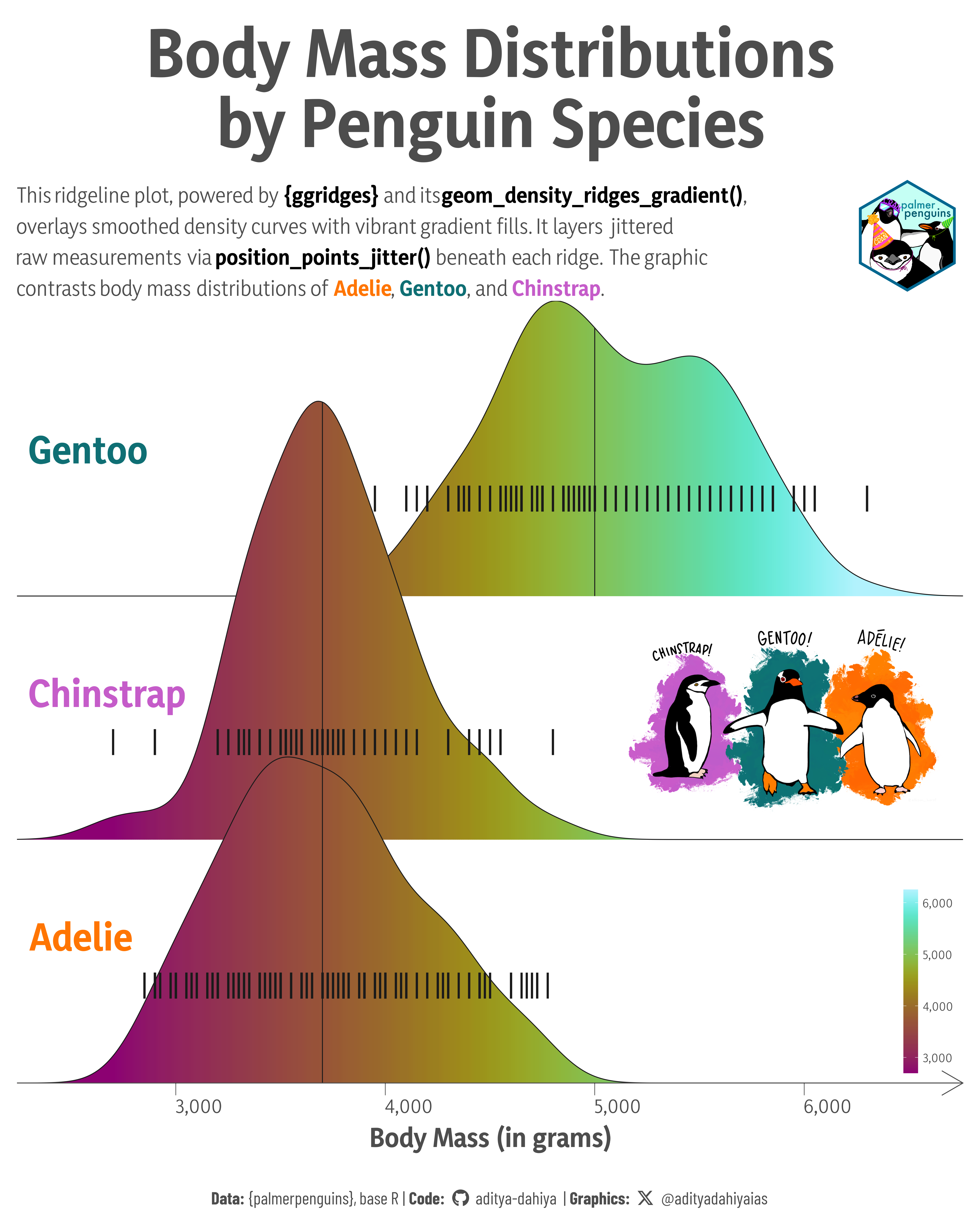
This plot uses ridgeline curves to compare the body mass distribution of Adelie, Gentoo, and Chinstrap penguins. It blends smooth density estimates with individual data points, using a color gradient to emphasize mass values and highlight species-specific differences in central tendency and spread.

About the Data

The penguins dataset is included in base R starting from version 4.5.0, and is available via the datasets package. It provides measurements of adult penguins across three species—Adélie, Chinstrap, and Gentoo—found on three islands in the Palmer Archipelago, Antarctica. Key variables include flipper length, body mass, bill dimensions, sex, and the year of observation. This dataset is a curated subset of a more extensive penguins_raw dataset, which also contains information on nesting behavior and blood isotope ratios. Originally used by Gorman et al. (2014) to explore sexual dimorphism in penguins, the dataset gained broader popularity through the palmerpenguins package as a user-friendly alternative to the classic iris dataset. Recent efforts by Kaye et al. (2025) have integrated this data directly into base R, along with reproducible scripts and documentation.

Figure 1: This graphic displays the distribution of body mass (in grams) across three species of penguins — Adelie, Gentoo, and Chinstrap — using ridgeline plots. Each ridge represents a smoothed density curve for a species, overlaid with individual data points and colored using a gradient based on body mass. The plot highlights differences in central tendency and spread, with Gentoo penguins generally being heavier, followed by Chinstrap and Adelie. Gradient shading emphasizes the mass range, while quantile lines indicate medians. This visualization effectively combines density estimation with raw data using the powerful {ggridges} extension to ggplot2.

How I made this graphic?

This ridgeline plot leverages the {ggridges} package to visualize body_mass distributions across three penguin species, using geom_density_ridges_gradient to apply a color gradient based on the underlying density. Statistical aesthetics such as stat(x) enable dynamic fill mapping, while quantile_lines = TRUE, quantiles = 2 highlights median density along each ridge (Vignette). Raw observations are overlaid via jittered points using position_points_jitter() for clarity, ensuring individual data points are visible beneath each curve. Manual species labels are added with geom_text(). A continuous palette from the {paletteer} package is applied with scale_fill_paletteer_c(), squishing values outside the specified limits for a polished color scale.

Loading required libraries

pacman::p_load(
  tidyverse,      # All tidy tools: data wrangling
  scales,         # Nice Scales for ggplot2
  fontawesome,    # Icons display in ggplot2
  ggtext,         # Markdown text support for ggplot2
  showtext,       # Display fonts in ggplot2
  colorspace,     # Lighten and Darken colours
  
  magick,         # Download images and edit them
  ggimage,        # Display images in ggplot2
  pactchwork,     # Composing Plots
  
  ggridges        # for ridgeline density plots
)


penguins <- penguins |> 
  as_tibble()

Visualization Parameters

# Font for titles
font_add_google("Yaldevi",
  family = "title_font"
) 

# Font for the caption
font_add_google("Barlow Condensed",
  family = "caption_font"
) 

# Font for plot text
font_add_google("Fira Code",
  family = "body_font"
) 

showtext_auto()

# cols4all::c4a_gui()
# Pick a colour paletter that is Colour-Blind friendly, fair and 
# has a good contrast ratio with white
mypal <- paletteer::paletteer_d("ltc::trio3")

mypal <- c("#FF7502", "#C55CC9", "#0F6F74")

# A base Colour
bg_col <- "white"
seecolor::print_color(bg_col)

# Colour for highlighted text
text_hil <- "grey30"
seecolor::print_color(text_hil)

# Colour for the text
text_col <- "grey30"
seecolor::print_color(text_col)

line_col <- "grey30"

# Define Base Text Size
bts <- 90

# Caption stuff for the plot
sysfonts::font_add(
  family = "Font Awesome 6 Brands",
  regular = here::here("docs", "Font Awesome 6 Brands-Regular-400.otf")
)
github <- "&#xf09b"
github_username <- "aditya-dahiya"
xtwitter <- "&#xe61b"
xtwitter_username <- "@adityadahiyaias"
social_caption_1 <- glue::glue("<span style='font-family:\"Font Awesome 6 Brands\";'>{github};</span> <span style='color: {text_hil}'>{github_username}  </span>")
social_caption_2 <- glue::glue("<span style='font-family:\"Font Awesome 6 Brands\";'>{xtwitter};</span> <span style='color: {text_hil}'>{xtwitter_username}</span>")
plot_caption <- paste0(
  "**Data:** {palmerpenguins}, base R", 
  " |  **Code:** ", 
  social_caption_1, 
  " |  **Graphics:** ", 
  social_caption_2
  )
rm(github, github_username, xtwitter, 
   xtwitter_username, social_caption_1, 
   social_caption_2)

# Add text to plot-------------------------------------------------
plot_title <- "Body Mass Distributions\nby Penguin Species"

plot_subtitle <- "This ridgeline plot, powered by <b style='color:black'>{ggridges}</b> and its<b style='color:black'>geom_density_ridges_gradient()</b>,<br>overlays smoothed density curves with vibrant gradient fills. It layers jittered<br>raw measurements via <b style='color:black'>position_points_jitter()</b> beneath each ridge. The graphic<br>contrasts body mass distributions of <b style='color:#FF7502'>Adelie</b>, <b style='color:#0F6F74'>Gentoo</b>, and <b style='color:#C55CC9'>Chinstrap</b>."

Exploratory Data Analysis and Wrangling

logo1 <- image_read("https://allisonhorst.github.io/palmerpenguins/reference/figures/lter_penguins.png") |> 
  image_background("transparent")

logo2 <- image_read("https://education.rstudio.com/blog/2020/07/palmerpenguins-cran/penguins_cran.png")

penguins |> 
  distinct(species) |> 
  pull() |> 
  as.character()

The Plot

g_base <- penguins |> 
  ggplot() +
  
  # Density Ridges with Fill Gradient
  geom_density_ridges_gradient(
    mapping = aes(
      x = body_mass,
      y = species,
      group = species,
      fill = stat(x)
    ),
    linewidth = 0.5,
    colour = "grey10",
    quantile_lines = TRUE,
    quantiles = 2,
    jittered_points = TRUE,
    position = position_points_jitter(
      width = 0.1, height = 0,
      yoffset = 0.4
      ),
    point_shape = "|", 
    point_size = 35, 
    point_alpha = 1
  ) +
  paletteer::scale_fill_paletteer_c(
    "scico::hawaii",
    limits = c(2700, 6250),
    oob = scales::squish,
    labels = scales::label_number(big.mark = ",")
  ) +
  
  # Add Y-Axis Labels manually on the plot
  geom_text(
    data = penguins |> distinct(species),
    mapping = aes(x = 2300, y = species, colour = species, label = species),
    nudge_y = 0.6,
    family = "title_font",
    fontface = "bold",
    size = bts * 0.5,
    hjust = 0
  ) +
  scale_colour_manual(
    values = mypal
  ) +
  
  # Add a penguins photo
  annotation_custom(
    grid::rasterGrob(logo1),
    xmin = 5100, xmax = 6700, 
    ymin = 2, ymax = 3
  ) +
  scale_x_continuous(
    expand = expansion(0),
    labels = scales::label_number(big.mark = ",")
  ) +
  scale_y_discrete(
    expand = expansion(c(0, 0.2))
  ) +
  labs(
    title = plot_title,
    subtitle = plot_subtitle,
    caption = plot_caption,
    fill = NULL,
    x = "Body Mass (in grams)",
    y = NULL
  ) +
  guides(
    colour = "none"
  ) +
  theme_minimal(
    base_family = "title_font",
    base_size = bts
  ) +
  theme(
    
    # Overall
    plot.margin = margin(5,5,5,5, "mm"),
    legend.position = "inside",
    plot.title.position = "plot",
    text = element_text(
      colour = text_col,
      lineheight = 0.3,
      hjust = 0.5
    ),
    
    # Labels and Strip Text
    plot.title = element_text(
      colour = text_hil,
      margin = margin(5,0,5,0, "mm"),
      size = bts * 2.5,
      lineheight = 0.3,
      hjust = 0.5,
      family = "title_font",
      face = "bold"
    ),
    plot.subtitle = element_textbox(
      colour = text_hil,
      margin = margin(5,0,0,0, "mm"),
      size = 0.8 * bts,
      lineheight = 0.5,
      hjust = 0,
      halign = 0,
      family = "title_font"
    ),
    plot.caption = element_textbox(
      margin = margin(15,0,0,0, "mm"),
      hjust = 0.5,
      colour = text_hil,
      size = 0.7 * bts,
      family = "caption_font"
    ),
    plot.caption.position = "plot",
    
    # Axes
    axis.line.x = element_line(
      colour = text_col,
      arrow = arrow(length = unit(10, "mm")),
      linewidth = 0.5
    ),
    axis.line.y = element_blank(),
    axis.ticks.x = element_line(linewidth = 0.25),
    axis.ticks.y = element_blank(),
    axis.ticks.length.x = unit(5, "mm"),
    axis.ticks.length.y = unit(0, "mm"),
    axis.title.x = element_text(
      margin = margin(2,0,0,0, "mm"),
      face = "bold"
    ),
    axis.title.y = element_blank(),
    axis.text.x = element_text(
      margin = margin(1,0,2,0, "mm"),
      hjust = 0
    ),
    axis.text.y = element_blank(),
    
    # Panel Grid
    panel.grid = element_blank(),
    
    # Legend.
    legend.position.inside = c(1, 0),
    legend.direction = "vertical",
    legend.title = element_blank(),
    legend.text = element_text(
      size = bts / 2,
      margin = margin(0,0,0,2, "mm")
    ),
    legend.justification = c(1, 0),
    legend.key.width = unit(6, "mm"),
    legend.key.height = unit(15, "mm"),
    legend.margin = margin(4,4,4,4, "mm"),
    legend.box.margin = margin(0,0,0,0, "mm")
  )

g_inset <- ggplot() +
  # Add a penguins photo
  annotation_custom(
    grid::rasterGrob(logo2),
    xmin = -Inf, xmax = Inf, 
    ymin = -Inf, ymax = Inf
  ) +
  theme_void()

g <- g_base +
  inset_element(
    p = g_inset,
    left = 0.88, right = 0.98,
    bottom = 0.74, top = 0.88,
    align_to = "full",
    clip = FALSE
  )
ggsave(
  filename = here::here(
    "data_vizs",
    "tidy_palmerpenguins_2.png"
  ),
  plot = g,
  width = 400,
  height = 500,
  units = "mm",
  bg = bg_col
)

Savings the thumbnail for the webpage

# Saving a thumbnail

library(magick)

# Saving a thumbnail for the webpage
image_read(here::here("data_vizs", 
                      "tidy_palmerpenguins_2.png")) |> 
  image_resize(geometry = "x400") |> 
  image_write(
    here::here(
      "data_vizs", 
      "thumbnails", 
      "tidy_palmerpenguins_2.png"
    )
  )

Session Info

pacman::p_load(
  tidyverse,      # All tidy tools: data wrangling
  scales,         # Nice Scales for ggplot2
  fontawesome,    # Icons display in ggplot2
  ggtext,         # Markdown text support for ggplot2
  showtext,       # Display fonts in ggplot2
  colorspace,     # Lighten and Darken colours
  
  magick,         # Download images and edit them
  ggimage,        # Display images in ggplot2
  pactchwork,     # Composing Plots
  
  ggridges        # for ridgeline density plots
)



sessioninfo::session_info()$packages |> 
  as_tibble() |> 
  select(package, 
         version = loadedversion, 
         date, source) |> 
  arrange(package) |> 
  janitor::clean_names(
    case = "title"
  ) |> 
  gt::gt() |> 
  gt::opt_interactive(
    use_search = TRUE
  ) |> 
  gtExtras::gt_theme_espn()

Table 1: R Packages and their versions used in the creation of this page and graphics