Animation in the Long Run: Pixar’s Increasing Movie Lengths

This analysis explores the increasing runtime of Pixar films using {ggplot2} for visualization, with enhancements from packages like {ggimage} for embedding movie posters.

About the Data

The data for this week’s #TidyTuesday comes from the {pixarfilms} R package by Eric Leung, which compiles information about Pixar films, their box office performance, critical reception, and ratings from sources like Wikipedia. The dataset includes two key files: pixar_films.csv, which details the release date, runtime, and rating of each film, and public_response.csv, which compiles critic and audience scores from platforms such as Rotten Tomatoes, Metacritic, and CinemaScore. Data can be accessed in R using the {tidytuesdayR} package or directly via read_csv(). This dataset offers opportunities to explore rating discrepancies, missing data patterns, and the relationship between box office earnings and film reviews.

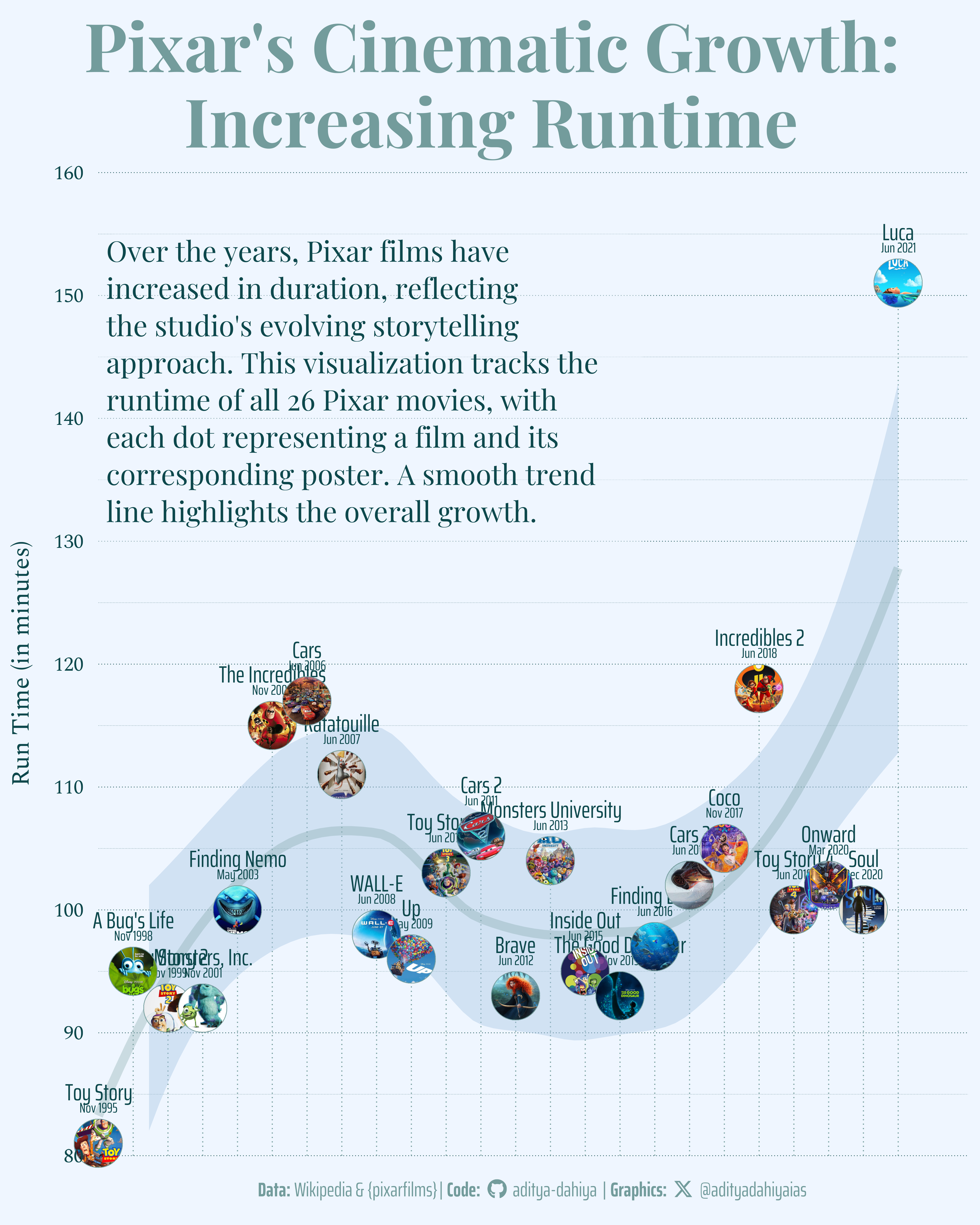
Figure 1: Each dot represents a Pixar film, positioned by its release year on the X-axis and its runtime (in minutes) on the Y-axis. The smooth line illustrates the overall trend of increasing film durations over time, with occasional fluctuations. Film posters provide a visual reference for each title. Data sourced from the {pixarfilms} R package, compiled from Wikipedia.

How I made this graphic?

Loading required libraries, data import & creating custom functions.

# Data Import and Wrangling Tools
library(tidyverse)            # All things tidy

# Final plot tools
library(scales)               # Nice Scales for ggplot2
library(fontawesome)          # Icons display in ggplot2
library(ggtext)               # Markdown text support for ggplot2
library(showtext)             # Display fonts in ggplot2
library(colorspace)           # Lighten and Darken colours

# Other Tools
library(ggpattern)            # Image patterns in ggplot2 geoms
library(magick)               # Handling images
library(httr)                 # Downloading images from Google

# Using R
pixar_films <- readr::read_csv('https://raw.githubusercontent.com/rfordatascience/tidytuesday/main/data/2025/2025-03-11/pixar_films.csv')
public_response <- readr::read_csv('https://raw.githubusercontent.com/rfordatascience/tidytuesday/main/data/2025/2025-03-11/public_response.csv')

Visualization Parameters

# Font for titles
font_add_google("Playfair Display",
  family = "title_font"
) 

# Font for the caption
font_add_google("Saira Extra Condensed",
  family = "caption_font"
) 

# Font for plot text
font_add_google("Spectral",
  family = "body_font"
) 

showtext_auto()

mypal <- paletteer::paletteer_d("rockthemes::zeppelin")
mypal2 <- paletteer::paletteer_d("trekcolors::enara2")

# A base Colour
bg_col <-colorspace::lighten("#BFCFE3FF", 0.8)
seecolor::print_color(bg_col)

# Colour for highlighted text
text_hil <- mypal[2]
seecolor::print_color(text_hil)

# Colour for the text
text_col <- mypal[3]
seecolor::print_color(text_col)


# Define Base Text Size
bts <- 90 

# Caption stuff for the plot
sysfonts::font_add(
  family = "Font Awesome 6 Brands",
  regular = here::here("docs", "Font Awesome 6 Brands-Regular-400.otf")
)
github <- "&#xf09b"
github_username <- "aditya-dahiya"
xtwitter <- "&#xe61b"
xtwitter_username <- "@adityadahiyaias"
social_caption_1 <- glue::glue("<span style='font-family:\"Font Awesome 6 Brands\";'>{github};</span> <span style='color: {text_hil}'>{github_username}  </span>")
social_caption_2 <- glue::glue("<span style='font-family:\"Font Awesome 6 Brands\";'>{xtwitter};</span> <span style='color: {text_hil}'>{xtwitter_username}</span>")
plot_caption <- paste0(
  "**Data:** Wikipedia & {pixarfilms}", 
  " |  **Code:** ", 
  social_caption_1, 
  " |  **Graphics:** ", 
  social_caption_2
  )
rm(github, github_username, xtwitter, 
   xtwitter_username, social_caption_1, 
   social_caption_2)

# Add text to plot-------------------------------------------------
plot_title <- "Pixar's Cinematic Growth:\nIncreasing Runtime"

plot_subtitle <- "Over the years, Pixar films have increased in duration, reflecting the studio's evolving storytelling approach. This visualization tracks the runtime of all 26 Pixar movies, with each dot representing a film and its corresponding poster. A smooth trend line highlights the overall growth."

Exploratory Data Analysis and Wrangling

# library(summarytools)
# pixar_films |> dfSummary() |> view()
# public_response |> dfSummary() |> view()
# 
# pixar_films |> 
#   ggplot(
#     aes(
#       x = release_date,
#       y = run_time
#     )
#   ) +
#   geom_point() +
#   geom_text(
#     aes(label = film)
#   )

df <- pixar_films |>
  mutate(id = row_number()) |> 
  left_join(public_response) |> 
  pivot_longer(
    cols = c(run_time, rotten_tomatoes, metacritic, critics_choice),
    names_to = "facet_var",
    values_to = "y_var"
  ) |> 
  mutate(
    facet_var = snakecase::to_title_case(facet_var),
    image_var = paste0("data_vizs/temp_pixar_films_", id, ".png")
  ) |> 
  filter(
    release_date < as_date("2023-01-01")
  )

levels_facet <- df$facet_var |> unique()

df <- df |> 
  mutate(facet_var = fct(facet_var, levels = levels_facet)) |> 
  filter(facet_var == "Run Time")

plotdf <- df |> 
  distinct(film)

Get images of Movie posters

# Get a custom google search engine and API key
# Tutorial: https://developers.google.com/custom-search/v1/overview
# Tutorial 2: https://programmablesearchengine.google.com/

# From:https://developers.google.com/custom-search/v1/overview
# google_api_key <- "LOAD YOUR GOOGLE API KEY HERE"

# From: https://programmablesearchengine.google.com/controlpanel/all
# my_cx <- "GET YOUR CUSTOM SEARCH ENGINE ID HERE"

# Load necessary packages
library(httr)
library(magick)

# Define function to download and save movie poster
download_icons <- function(i) {
  
  api_key <- google_api_key
  cx <- my_cx
  
  # Build the API request URL
  url <- paste0("https://www.googleapis.com/customsearch/v1?q=", 
                URLencode(paste0(plotdf$film[i], " movie poster")), 
                "&cx=", cx, 
                "&searchType=image&key=", api_key)
  
  # Make the request
  response <- GET(url)
  result <- content(response, "parsed")
  
  # Get the URL of the first image result
  image_url <- result$items[[1]]$link
  
  magick::image_read(image_url) |> 
    image_resize("x300") |> 
    cropcircles::circle_crop(
      border_size = 3,
      border_colour = text_hil
    ) |> 
    image_read() |> 
    image_write(
      here::here(
        "data_vizs",
        paste0("temp_pixar_films_", i,".png"))
    )
}

for (i in 1:nrow(plotdf)) {
  download_icons(i)
}

The Base Plot

g <- ggplot(
  data = df,
  mapping = aes(
    x = number,
    y = y_var
  )
) +
  geom_segment(
    mapping = aes(
      y = 80,
      xend = number,
      yend = y_var
    ),
    colour = text_hil,
    linetype = 3,
    linewidth = 0.6
  ) +
  geom_smooth(
    mapping = aes(
    group = facet_var
    ),
    fill = darken(bg_col, 0.2),
    se = TRUE,
    linewidth = 5,
    colour = alpha(text_hil, 0.3)
  ) +
  geom_point(size = 15, alpha = 0.2) +
  geom_text(
    mapping = aes(
      label = film
    ),
    family = "caption_font",
    colour = text_col,
    nudge_y = 3.5,
    hjust = 0.5,
    vjust = 0,
    size = bts / 3
  ) +
  geom_text(
    mapping = aes(
      label = format(release_date, "%b %Y")
    ),
    family = "caption_font",
    colour = text_col,
    nudge_y = 3.3,
    hjust = 0.5,
    vjust = 1,
    size = bts / 5
  ) +
  ggimage::geom_image(
    mapping = aes(
      image = image_var
    ),
    size = 0.05
  ) +
  annotate(
    geom = "label",
    x = 1,
    y = 155,
    hjust = 0,
    vjust = 1,
    label = str_wrap(plot_subtitle, 40),
    family = "title_font",
    size = bts / 2.5,
    fill = alpha(bg_col, 0.5),
    lineheight = 0.35,
    label.size = NA,
    colour = text_col
  ) +
  labs(
    title = plot_title,
    caption = plot_caption,
    x = NULL,
    y = "Run Time (in minutes)"
  ) +
  scale_x_continuous(expand = expansion(0)) +
  scale_y_continuous(
    expand = expansion(0),
    limits = c(80, 160),
    breaks = seq(80, 160, 10)
  ) +
  scale_colour_manual(values = mypal2) +
  coord_cartesian(
    clip = "off"
  ) +
  # facet_wrap(
  #   ~facet_var,
  #   ncol = 1,
  #   scales = "free_y"
  # ) +
  theme_minimal(
    base_family = "body_font",
    base_size = bts
  ) +
  theme(
    
    # Overall Plot
    legend.position = "none", 
    plot.margin = margin(5,5,5,5, "mm"),
    plot.title.position = "plot",
    panel.grid = element_line(
      linetype = 3,
      linewidth = 0.4,
      colour = text_col
    ),
    panel.grid.major.x = element_blank(),
    panel.grid.minor.x = element_blank(),
    axis.ticks = element_blank(),
    axis.ticks.length = unit(0, "mm"),
    text = element_text(
      colour = text_col,
      margin = margin(0,0,0,0, "mm"),
      hjust = 0.5,
      vjust = 0.5,
      lineheight = 0.3
    ),
    
    # Axis Text
    axis.text = element_text(
      margin = margin(0,0,0,0, "mm"),
      colour = text_col
    ),
    axis.text.x = element_blank(),
    axis.title = element_text(
      margin = margin(0,0,0,0, "mm"),
      colour = text_col
    ),
    
    # Labels and Strip Text
    plot.title = element_text(
      colour = text_hil,
      margin = margin(5,0,5,0, "mm"),
      size = bts * 2.7,
      lineheight = 0.3,
      hjust = 0.5,
      family = "title_font",
      face = "bold"
    ),
    plot.caption = element_textbox(
      family = "caption_font",
      margin = margin(10,0,5,0, "mm"),
      hjust = 0.5,
      colour = text_hil
    ),
    
    # Facets and Strips
    panel.spacing.y = unit(2, "mm"),
    strip.text = element_text(
      margin = margin(5,0,0,0, "mm"),
      family = "body_font",
      hjust = 0,
      size = 2 * bts,
      colour = text_col
    ),
    panel.background = element_rect(
      fill = "transparent",
      colour = "transparent",
      linewidth = 0
    )
  )

ggsave(
  filename = here::here(
    "data_vizs",
    "tidy_pixar_films.png"
  ),
  plot = g,
  width = 400,
  height = 500,
  units = "mm",
  bg = bg_col
)

Reduce filesize and Savings the thumbnail for the webpage

list.files(
  path = "data_vizs", 
  pattern = "^temp_pixar_films", 
  full.names = TRUE
  )

file.remove(
  list.files(
    path = "data_vizs", 
    pattern = "^temp_pixar_films", 
    full.names = TRUE
  )
)

# Saving a thumbnail

library(magick)
# Saving a thumbnail for the webpage
image_read(here::here("data_vizs", 
                      "tidy_pixar_films.png")) |> 
  image_resize(geometry = "x400") |> 
  image_write(
    here::here(
      "data_vizs", 
      "thumbnails", 
      "tidy_pixar_films.png"
    )
  )

Session Info

# Data Import and Wrangling Tools
library(tidyverse)            # All things tidy

# Final plot tools
library(scales)               # Nice Scales for ggplot2
library(fontawesome)          # Icons display in ggplot2
library(ggtext)               # Markdown text support for ggplot2
library(showtext)             # Display fonts in ggplot2
library(colorspace)           # Lighten and Darken colours
library(ggpattern)            # Image patterns in ggplot2 geoms
library(magick)               # Handling images
library(httr)                 # Downloading images from Google

sessioninfo::session_info()$packages |> 
  as_tibble() |> 
  select(package, 
         version = loadedversion, 
         date, source) |> 
  arrange(package) |> 
  janitor::clean_names(
    case = "title"
  ) |> 
  gt::gt() |> 
  gt::opt_interactive(
    use_search = TRUE
  ) |> 
  gtExtras::gt_theme_espn()

Table 1: R Packages and their versions used in the creation of this page and graphics