Common words in talks during posit::conf (2023-24)

Wordclouds showing the common words during the talks given in posit::conf

About the Data

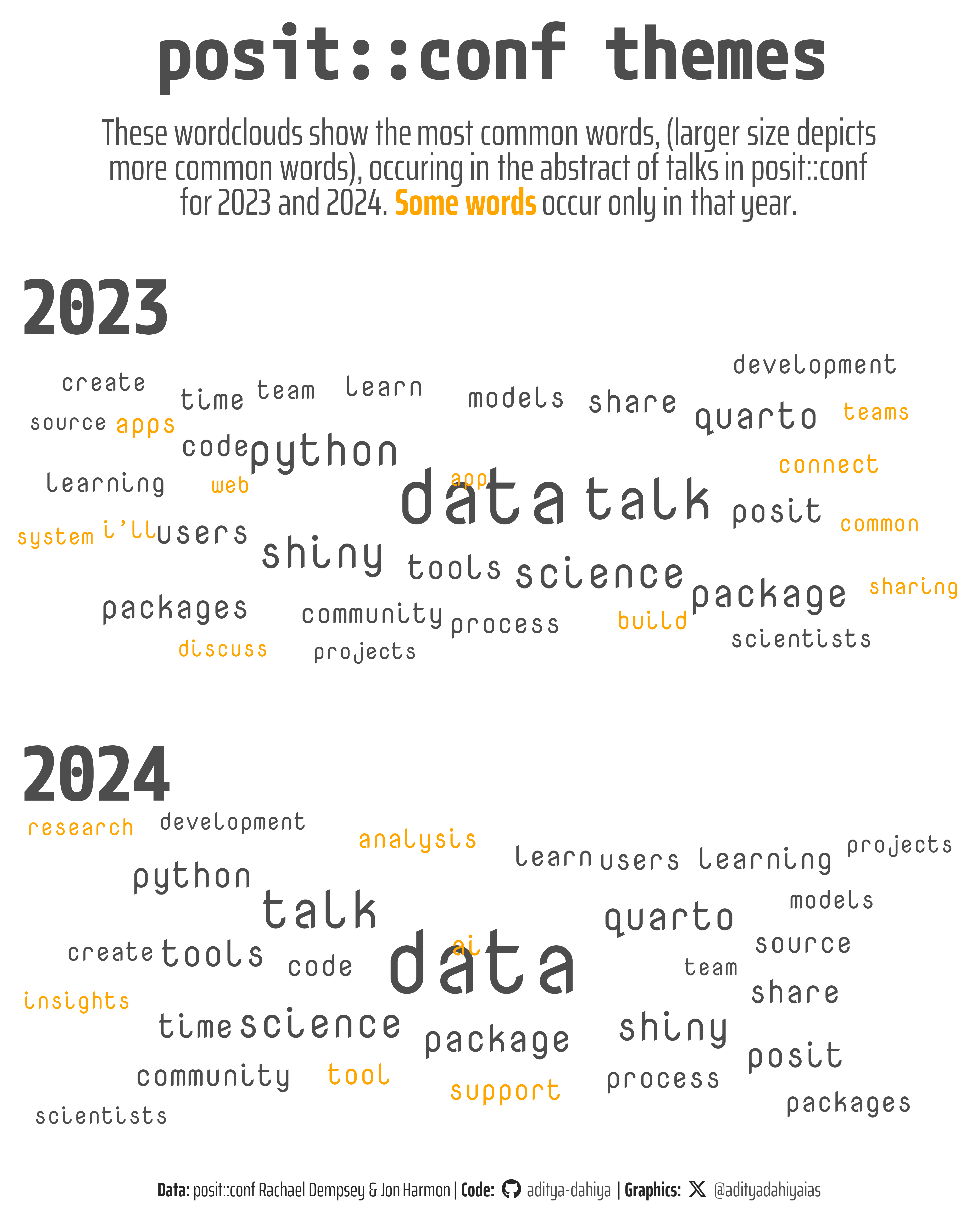
The dataset on posit::conf talks provides insights into sessions held during posit::conf in 2023 and 2024, focusing on R and Python programming languages and their applications in data science. The data was curated by Jon Harmon and includes speaker details, session types, track titles, and abstracts for 2023, as well as YouTube links for 2024 talks. This information allows exploration of recurring speakers, shared themes, and sentiment analysis across the event’s tracks. The data is accessible through the tidytuesdayR package or directly via GitHub links.

Figure 1: Two wordclouds, one each for 2023 and 2024, and the size of words represents the commonness of the word during that year. The orange words represent words that occurred only during that year.

How I made this graphic?

Loading required libraries, data import & creating custom functions.

# Data Import and Wrangling Tools
library(tidyverse)            # All things tidy

# Final plot tools
library(scales)               # Nice Scales for ggplot2
library(fontawesome)          # Icons display in ggplot2
library(ggtext)               # Markdown text support for ggplot2
library(showtext)             # Display fonts in ggplot2
library(colorspace)           # Lighten and Darken colours
library(patchwork)            # Compiling Plots
library(tidytext)             # Getting words analysis in R
library(ggwordcloud)          # Creating Word-Clouds with ggplot2

# Option 2: Read directly from GitHub

conf2023 <- readr::read_csv('https://raw.githubusercontent.com/rfordatascience/tidytuesday/main/data/2025/2025-01-14/conf2023.csv')
conf2024 <- readr::read_csv('https://raw.githubusercontent.com/rfordatascience/tidytuesday/main/data/2025/2025-01-14/conf2024.csv')

Visualization Parameters

# Font for titles
font_add_google("M PLUS 1 Code",
  family = "title_font"
) 

# Font for the caption
font_add_google("Saira Extra Condensed",
  family = "caption_font"
) 

# Font for plot text
font_add_google("Nova Mono",
  family = "body_font"
) 

showtext_auto()

# A base Colour
bg_col <- "white"
seecolor::print_color(bg_col)

# Colour for highlighted text
text_hil <- "grey30"
seecolor::print_color(text_hil)

# Colour for the text
text_col <- "grey15"
seecolor::print_color(text_col)


# Define Base Text Size
bts <- 90 

# Caption stuff for the plot
sysfonts::font_add(
  family = "Font Awesome 6 Brands",
  regular = here::here("docs", "Font Awesome 6 Brands-Regular-400.otf")
)
github <- "&#xf09b"
github_username <- "aditya-dahiya"
xtwitter <- "&#xe61b"
xtwitter_username <- "@adityadahiyaias"
social_caption_1 <- glue::glue("<span style='font-family:\"Font Awesome 6 Brands\";'>{github};</span> <span style='color: {text_hil}'>{github_username}  </span>")
social_caption_2 <- glue::glue("<span style='font-family:\"Font Awesome 6 Brands\";'>{xtwitter};</span> <span style='color: {text_hil}'>{xtwitter_username}</span>")
plot_caption <- paste0(
  "**Data:** posit::conf   Rachael Dempsey & Jon Harmon", 
  " |  **Code:** ", 
  social_caption_1, 
  " |  **Graphics:** ", 
  social_caption_2
  )
rm(github, github_username, xtwitter, 
   xtwitter_username, social_caption_1, 
   social_caption_2)

# Add text to plot-------------------------------------------------
plot_title <- "posit::conf themes"

plot_subtitle <- "These wordclouds show the most common words, (larger size depicts<br>more common words), occuring in the abstract of talks in posit::conf<br>for 2023 and 2024. <b style='color:orange'>Some words</b> occur only in that year."

Exploratory Data Analysis and Wrangling

data("stop_words")

number_to_display <- 30

df1 <- bind_rows(
  conf2023 |> 
    select(session_abstract) |> 
    rename(text = session_abstract) |> 
    mutate(year = 2023) |> 
    distinct(),

  conf2024 |> 
    select(description) |> 
    rename(text = description) |> 
    mutate(year = 2024) |> 
    distinct()
)

df2 <- df1 |> 
  tidytext::unnest_tokens(output = "word", input = text) |> 
  anti_join(stop_words) |> 
  group_by(year) |> 
  count(word, sort = T) |> 
  slice_max(order_by = n, n = number_to_display)

words_2023 <- df2 |> 
  filter(year == 2023) |> 
  pull(word)

words_2024 <- df2 |> 
  filter(year == 2024) |> 
  pull(word)

plotdf <- df2 |> 
  mutate(
    colour_var = case_when(
      (year == 2023) & !(word %in% words_2024) ~ "Highlight",
      (year == 2024) & !(word %in% words_2023) ~ "Highlight",
      .default = "Others"
    )
  )

The Base Plot

set.seed(3)
g <- plotdf |> 
  mutate(
    angle_var = 45 * sample(-2:2, n(),
                            replace = TRUE,
                            prob = c(1, 1, 4, 1, 1)
                            )
  ) |>
  ggplot() +
  ggwordcloud::geom_text_wordcloud(
    mapping = aes(
      label = word,
      size = n,
      colour = colour_var
    ),
    family = "body_font",
    fontface = "bold",
    rm_outside = TRUE,
    shape = "square",
    eccentricity = 0.8,
    # grid_size = 8,
    grid_margin = 3,
    seed = 6
  ) +
  scale_colour_manual(
    values = c("orange", text_hil)
  ) +
  scale_size_area(
    max_size = bts * 1.25, 
    trans = power_trans(1)
  ) +
  facet_wrap(~year, ncol = 1) +
  coord_cartesian(clip = "off") +
  labs(
    title = plot_title,
    subtitle = plot_subtitle,
    caption = plot_caption
  ) +
  
  theme_minimal(
    base_family = "body_font",
    base_size = bts
  ) +
  theme(
    
    # Overall Plot
    plot.margin = margin(0,0,0,0, "mm"),
    plot.title.position = "plot",
    panel.spacing = unit(0, "mm"),
    text = element_text(
      colour = text_col,
      margin = margin(0,0,0,0, "mm"),
      hjust = 0.5,
      vjust = 0.5,
      lineheight = 0.3
    ),
    
    # Labels and Strip Text
    plot.title = element_text(
      colour = text_hil,
      margin = margin(10,0,5,0, "mm"),
      size = bts * 3,
      lineheight = 0.3,
      hjust = 0.5,
      face = "bold",
      family = "title_font"
    ),
    plot.subtitle = element_textbox(
      colour = text_hil,
      margin = margin(5,0,10,0, "mm"),
      size = bts * 1.5,
      hjust = 0.5,
      halign = 0.5,
      lineheight = 0.3,
      family = "caption_font"
    ),
    plot.caption = element_textbox(
      family = "caption_font",
      margin = margin(0,0,10,0, "mm"),
      hjust = 0.5
    ),
    strip.text = element_text(
      family = "title_font",
      colour = text_hil,
      size = bts * 3,
      margin = margin(10,0,-20,10, "mm"),
      face = "bold",
      hjust = 0
    ),
    panel.background = element_rect(
      fill = "transparent",
      colour = "transparent"
    )
  )

ggsave(
  filename = here::here(
    "data_vizs",
    "tidy_posit_conf.png"
  ),
  plot = g,
  width = 400,
  height = 500,
  units = "mm",
  bg = bg_col
)

Savings the thumbnail for the webpage

# Saving a thumbnail

library(magick)
# Saving a thumbnail for the webpage
image_read(here::here("data_vizs", 
                      "tidy_posit_conf.png")) |> 
  image_resize(geometry = "x400") |> 
  image_write(
    here::here(
      "data_vizs", 
      "thumbnails", 
      "tidy_posit_conf.png"
    )
  )

Session Info

# Data Import and Wrangling Tools
library(tidyverse)            # All things tidy

# Final plot tools
library(scales)               # Nice Scales for ggplot2
library(fontawesome)          # Icons display in ggplot2
library(ggtext)               # Markdown text support for ggplot2
library(showtext)             # Display fonts in ggplot2
library(colorspace)           # Lighten and Darken colours
library(patchwork)            # Compiling Plots
library(tidytext)             # Getting words analysis in R
library(ggwordcloud)          # Creating Word-Clouds with ggplot2

sessioninfo::session_info()$packages |> 
  as_tibble() |> 
  select(package, 
         version = loadedversion, 
         date, source) |> 
  arrange(package) |> 
  janitor::clean_names(
    case = "title"
  ) |> 
  gt::gt() |> 
  gt::opt_interactive(
    use_search = TRUE
  ) |> 
  gtExtras::gt_theme_espn()

Table 1: R Packages and their versions used in the creation of this page and graphics