A Century-wise Look at Literary Language Trends

Stacked bar visualization of language proportions in Project Gutenberg books by author birth century.

#TidyTuesday

Bar Chart

Author

Aditya Dahiya

Published

July 9, 2025

About the Data

This week’s dataset, curated by Jon Harmon for the TidyTuesday project (week of June 3, 2025), features rich metadata from Project Gutenberg, the oldest digital library of public domain texts. The data is accessed using the {gutenbergr} R package, which allows users to search, download, and analyze tens of thousands of public domain works. The dataset is split across four CSV files: gutenberg_authors.csv, gutenberg_languages.csv, gutenberg_metadata.csv, and gutenberg_subjects.csv. These files include detailed information on author identities and aliases, language availability (using ISO 639 language codes), book titles, bookshelf classifications, and Library of Congress Subject Headings (LCSH). The dataset supports multilingual analysis, investigation into author duplication via gutenberg_author_id, and potential improvements to metadata curation. Whether you’re using R, Python, or Julia, the data can be accessed either via TidyTuesday libraries or directly from the GitHub repository.

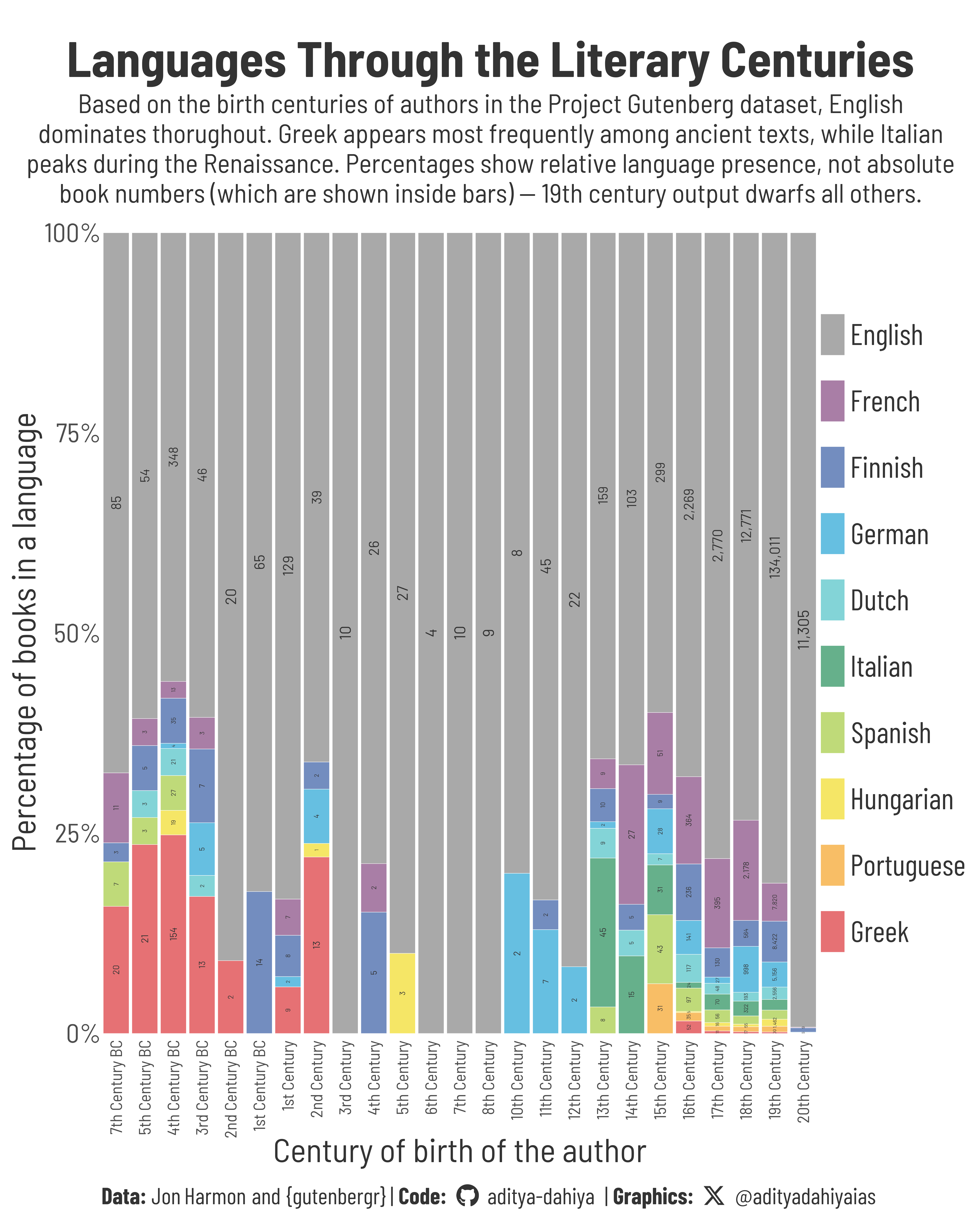
Figure 1: Books from Project Gutenberg are grouped by the authors’ birth centuries, with stacked bars showing the proportion of books in each of the ten most frequent languages. Percentages are within-century distributions. The absolute number of books is shown as text inside the bars.

How the Graphic Was Created

To explore historical language patterns in public domain books, I used data from Project Gutenberg via the {gutenbergr} R package, curated for the TidyTuesday project (2025-06-03) by Jon Harmon. The analysis focused on authors’ birth centuries and the languages in which their works appear in the Project Gutenberg collection.

Key Findings

English has consistently dominated the corpus, especially from the 18th century onward.
Greek emerges prominently among authors born between the 7th century BC and 2nd century AD, reflecting the enduring legacy of classical texts.
Italian saw a notable rise in the 13th and 14th centuries, likely due to the cultural flowering during the Italian Renaissance.
The graphic displays relative proportions of languages by century (not absolute counts). The actual number of books by authors born in the 19th century far exceeds those from all earlier periods combined.

Tools & Techniques

This visual was created in R using the ggplot2 ecosystem. The full pipeline included:

Data wrangling with tidyverse, dplyr, and forcats
Enhanced fonts using showtext and Google Fonts like Barlow
Aesthetics and themes customized via ggtext, colorspace, and patchwork
Font Awesome icons were embedded in the caption using the fontawesome R package
The final plot was saved using ggsave(), with careful control over typography, spacing, and layout.

Authors’ birth years were used to compute the century of birth, which was then plotted along the x-axis. Each bar represents the percentage distribution of books in different languages per century. For clarity, language codes (like en, el, it) were translated into full language names.

The visualization offers a compelling lens into the temporal geography of literature—revealing how languages like Greek and Italian peaked during classical and early Renaissance eras, while English has seen sustained growth over the centuries.

View the graphic on GitHub or follow updates on X/Twitter. Data: {gutenbergr} • Code and Visualization: Aditya Dahiya

Loading required libraries

Code

pacman::p_load(
  tidyverse,            # All things tidy
  
  scales,               # Nice Scales for ggplot2
  fontawesome,          # Icons display in ggplot2
  ggtext,               # Markdown text support for ggplot2
  showtext,             # Display fonts in ggplot2
  colorspace,           # Lighten and Darken colours

  patchwork             # Composing Plots
)

gutenberg_authors <- readr::read_csv('https://raw.githubusercontent.com/rfordatascience/tidytuesday/main/data/2025/2025-06-03/gutenberg_authors.csv')

gutenberg_languages <- readr::read_csv('https://raw.githubusercontent.com/rfordatascience/tidytuesday/main/data/2025/2025-06-03/gutenberg_languages.csv')

gutenberg_metadata <- readr::read_csv('https://raw.githubusercontent.com/rfordatascience/tidytuesday/main/data/2025/2025-06-03/gutenberg_metadata.csv')

gutenberg_subjects <- readr::read_csv('https://raw.githubusercontent.com/rfordatascience/tidytuesday/main/data/2025/2025-06-03/gutenberg_subjects.csv')

Visualization Parameters

Code

# Font for titles
font_add_google("Barlow",
  family = "title_font"
) 

# Font for the caption
font_add_google("Barlow Condensed",
  family = "caption_font"
) 

# Font for plot text
font_add_google("Barlow Semi Condensed",
  family = "body_font"
) 

showtext_auto()

# A base Colour
bg_col <- "white"
seecolor::print_color(bg_col)

# Colour for highlighted text
text_hil <- "grey20"
seecolor::print_color(text_hil)

# Colour for the text
text_col <- "grey20"
seecolor::print_color(text_col)

line_col <- "grey30"

# Define Base Text Size
bts <- 120

# Caption stuff for the plot
sysfonts::font_add(
  family = "Font Awesome 6 Brands",
  regular = here::here("docs", "Font Awesome 6 Brands-Regular-400.otf")
)
github <- "&#xf09b"
github_username <- "aditya-dahiya"
xtwitter <- "&#xe61b"
xtwitter_username <- "@adityadahiyaias"
social_caption_1 <- glue::glue("<span style='font-family:\"Font Awesome 6 Brands\";'>{github};</span> <span style='color: {text_hil}'>{github_username}  </span>")
social_caption_2 <- glue::glue("<span style='font-family:\"Font Awesome 6 Brands\";'>{xtwitter};</span> <span style='color: {text_hil}'>{xtwitter_username}</span>")
plot_caption <- paste0(
  "**Data:** Jon Harmon and {gutenbergr}", 
  " |  **Code:** ", 
  social_caption_1, 
  " |  **Graphics:** ", 
  social_caption_2
  )
rm(github, github_username, xtwitter, 
   xtwitter_username, social_caption_1, 
   social_caption_2)

# Add text to plot-------------------------------------------------
plot_subtitle <- str_wrap("Based on the birth centuries of authors in the Project Gutenberg dataset, English dominates thorughout. Greek appears most frequently among ancient texts, while Italian peaks during the Renaissance. Percentages show relative language presence, not absolute book numbers (which are shown inside bars) — 19th century output dwarfs all others.", 90)
str_view(plot_subtitle)

plot_title <- "Languages Through the Literary Centuries"

Exploratory Data Analysis and Wrangling

Code

pacman::p_load(summarytools)

dfSummary(gutenberg_authors) |> view()

dfSummary(gutenberg_languages) |> view()

gutenberg_metadata |> dfSummary() |> view()

gutenberg_subjects |> dfSummary() |> view()

df1 <- gutenberg_metadata |> 
  select(gutenberg_id, language) |> 
  left_join(
    gutenberg_subjects |> 
      select(gutenberg_id, subject),
    relationship = "many-to-many"
  ) |> 
  drop_na()

df1 |> 
  count(language, subject, sort = T)

df2 <- gutenberg_metadata |> 
  select(gutenberg_id, gutenberg_author_id,
         language) |> 
  left_join(
    gutenberg_subjects |> 
      select(gutenberg_id, subject),
    relationship = "many-to-many"
  ) |> 
  left_join(
    gutenberg_authors |> 
      select(gutenberg_author_id, author, birthdate, deathdate)
  ) |> 
  filter(!is.na(birthdate) & !is.na(deathdate)) |> 
  mutate(
    century = (birthdate%/%100) + 1
  ) |> 
  separate_longer_delim(language, "/") |> 
  mutate(
    language = fct(language),
    language = fct_lump_n(language, n = 10)
  ) |> 
  
  # Code assist by Claude Sonnet 4
  mutate(
    # Convert language codes to full names
    language = case_when(
      language == "en" ~ "English",
      language == "de" ~ "German",
      language == "fr" ~ "French",
      language == "it" ~ "Italian",
      language == "es" ~ "Spanish",
      language == "pt" ~ "Portuguese",
      language == "nl" ~ "Dutch",
      language == "fi" ~ "Finnish",
      language == "el" ~ "Greek",
      language == "hu" ~ "Hungarian",
      TRUE ~ "Others"  # Default case for any other values
    ),
    
    # Convert century numbers to formatted strings
    century = case_when(
      century < 0 ~ paste0(abs(century), case_when(
        abs(century) %% 10 == 1 & abs(century) %% 100 != 11 ~ "st",
        abs(century) %% 10 == 2 & abs(century) %% 100 != 12 ~ "nd",
        abs(century) %% 10 == 3 & abs(century) %% 100 != 13 ~ "rd",
        TRUE ~ "th"
      ), " Century BC"),
      century > 0 ~ paste0(century, case_when(
        century %% 10 == 1 & century %% 100 != 11 ~ "st",
        century %% 10 == 2 & century %% 100 != 12 ~ "nd",
        century %% 10 == 3 & century %% 100 != 13 ~ "rd",
        TRUE ~ "th"
      ), " Century"),
      TRUE ~ "Unknown"
    )
  ) |> 
  
  # Create ordered factor for century from oldest to newest
  mutate(
    century = factor(
      century, 
      levels = c(
        paste0(
          7:1, 
          c("th", "th", "th", "th", "rd", "nd", "st"), " Century BC"),
          paste0(
            1:20, 
            c("st", "nd", "rd", rep("th", 17)), 
            " Century"
            )
        ),
        ordered = TRUE)
  ) |> 
  filter(language != "Others")

language_levels <- df2 |> 
  count(language, sort = T) |> 
  pull(language)

plotdf <- df2 |> 
  filter(!is.na(century)) |> 
  count(century, language) |> 
  group_by(century) |> 
  mutate(
    perc = n / sum(n),
    language = fct(language, levels = language_levels)
  )

The Plot

Code

g <- plotdf |> 
  ggplot(
    aes(
      x = century,
      y = n,
      fill = language
    )
  ) +
  geom_col(
    position = position_fill(), 
    colour = bg_col,
    linewidth = 0.2,
    alpha = 0.6
  ) +
  geom_text(
    mapping = aes(
      label = number(n, big.mark = ","), 
      size = perc
    ),
    colour = text_col,
    position = position_fill(
      vjust = 0.5
    ),
    angle = 90,
    family = "title_font",
    check_overlap = TRUE
  ) +
  scale_y_continuous(
    expand = expansion(0),
    labels = label_percent()
  ) +
  scale_size(range = c(5, 20)) +
  # paletteer::scale_fill_paletteer_d("basetheme::royal") +
  paletteer::scale_fill_paletteer_d(
    "ggsci::default_frontiers",
    direction = -1
  ) +
  labs(
    fill = NULL,
    y = "Percentage of books in a language",
    x = "Century of birth of the author",
    title = plot_title,
    subtitle = plot_subtitle,
    caption = plot_caption
  ) +
  guides(
    size = "none"
  ) +
  theme_minimal(
    base_family = "body_font",
    base_size = bts
  ) +
  theme(
    
    # Overall
    text = element_text(
      margin = margin(0,0,0,0, "mm"),
      colour = text_col,
      lineheight = 0.3
    ),
    
    # Labels and Strip Text
    plot.title = element_text(
      margin = margin(10,0,0,0, "mm"),
      hjust = 0.5,
      vjust = 0.5,
      colour = text_hil,
      size = 1.5 * bts,
      family = "body_font",
      face = "bold"
      ),
    plot.subtitle = element_text(
      margin = margin(5,0,10,0, "mm"),
      hjust = 0.5,
      colour = text_hil,
      size = 0.8 * bts,
      family = "body_font"
    ),
    plot.caption = element_textbox(
      margin = margin(5,0,0,0, "mm"),
      hjust = 0.5,
      halign = 0.5,
      colour = text_hil,
      size = 0.7 * bts,
      family = "caption_font",
      fill = alpha("white", 0.6),
      box.color = NA,
      padding = unit(0.3, "lines"),
      r = unit(5, "mm")
    ),
    plot.caption.position = "plot",
    plot.title.position = "plot",
    plot.margin = margin(5,5,5,5, "mm"),
    
    
    # Legend
    legend.position = "right",
    legend.justification = c(0, 0.5),
    legend.direction = "vertical",
    legend.text.position = "right",
    legend.title.position = "top",
    
    legend.title = element_text(
      margin = margin(0,0,0,0, "mm"),
      hjust = 0.5,
      lineheight = 0.3,
      family = "body_font"
    ),
    legend.text = element_text(
      margin = margin(3,0,3,3, "mm"),
      size = bts * 0.9,
      family = "caption_font"
    ),
    legend.key.spacing.y = unit(10, "mm"),
    legend.margin = margin(0,0,0,0, "mm"),
    legend.box.spacing = unit(0, "mm"),
    legend.box.margin = margin(0,0,0,0, "mm"),
    legend.background = element_rect(
      fill = NA, colour = NA
    ),
    legend.key.width = unit(10, "mm"),
    legend.spacing.y = unit(10, "mm"),
    
    # Axes
    axis.ticks.length = unit(0, "mm"),
    axis.ticks = element_blank(),
    panel.grid = element_blank(),
    axis.line = element_blank(),
    axis.title.y = element_text(
      margin = margin(0,0,0,0, "mm"),
      hjust = 0.5
    ),
    axis.title.x = element_text(
      margin = margin(0,0,0,0, "mm"),
      hjust = 0.5
    ),
    axis.text.y = element_text(
      margin = margin(0,0,0,0, "mm")
    ),
    axis.text.x = element_text(
      margin = margin(3,0,0,0, "mm"),
      angle = 90,
      vjust = 0.5,
      hjust = 1,
      size = 0.5 * bts
    )
  )

ggsave(
  filename = here::here(
    "data_vizs",
    "tidy_project_gutenberg.png"
  ),
  plot = g,
  width = 400,
  height = 500,
  units = "mm",
  bg = bg_col
)

Savings the thumbnail for the webpage

Code

# Saving a thumbnail

library(magick)

# Saving a thumbnail for the webpage
image_read(here::here("data_vizs", 
                      "tidy_project_gutenberg.png")) |> 
  image_resize(geometry = "x400") |> 
  image_write(
    here::here(
      "data_vizs", 
      "thumbnails", 
      "tidy_project_gutenberg.png"
    )
  )

Session Info

Code

pacman::p_load(
  tidyverse,            # All things tidy
  
  scales,               # Nice Scales for ggplot2
  fontawesome,          # Icons display in ggplot2
  ggtext,               # Markdown text support for ggplot2
  showtext,             # Display fonts in ggplot2
  colorspace,           # Lighten and Darken colours

  patchwork             # Composing Plots
)

sessioninfo::session_info()$packages |> 
  as_tibble() |> 
  dplyr::select(package, 
         version = loadedversion, 
         date, source) |> 
  dplyr::arrange(package) |> 
  janitor::clean_names(
    case = "title"
  ) |> 
  gt::gt() |> 
  gt::opt_interactive(
    use_search = TRUE
  ) |> 
  gtExtras::gt_theme_espn()

Table 1: R Packages and their versions used in the creation of this page and graphics