Using geom_beeswarm() for visualization of price distributions across vehicle types
#TidyTuesday
{ggbeeswarm}
Author
Aditya Dahiya
Published
December 22, 2025
About the Data
The Qatar Cars dataset provides a modern, internationally-focused alternative to classic automotive datasets like mtcars and mpg. Collected in early 2025 by Paul Musgrave and students in his international politics course at Georgetown University in Qatar, this dataset addresses “U.S. defaultism” in data science education by using International System (SI) units, featuring globally diverse car manufacturers including Chinese brands, and incorporating modern vehicle types like electric and hybrid cars. The dataset includes 2025 prices in Qatari Riyals (QAR), with exchange rates of 1 USD = 3.64 QAR and 1 EUR = 4.15 QAR at the time of collection. Available through the {qatarcars} R package and as part of #TidyTuesday, the dataset contains 15 variables covering car specifications (dimensions in meters, mass in kilograms), performance metrics (horsepower, 0-100 km/h acceleration time), economic factors (fuel economy in liters per 100 km, price), and categorical information (origin country, engine type, vehicle type).
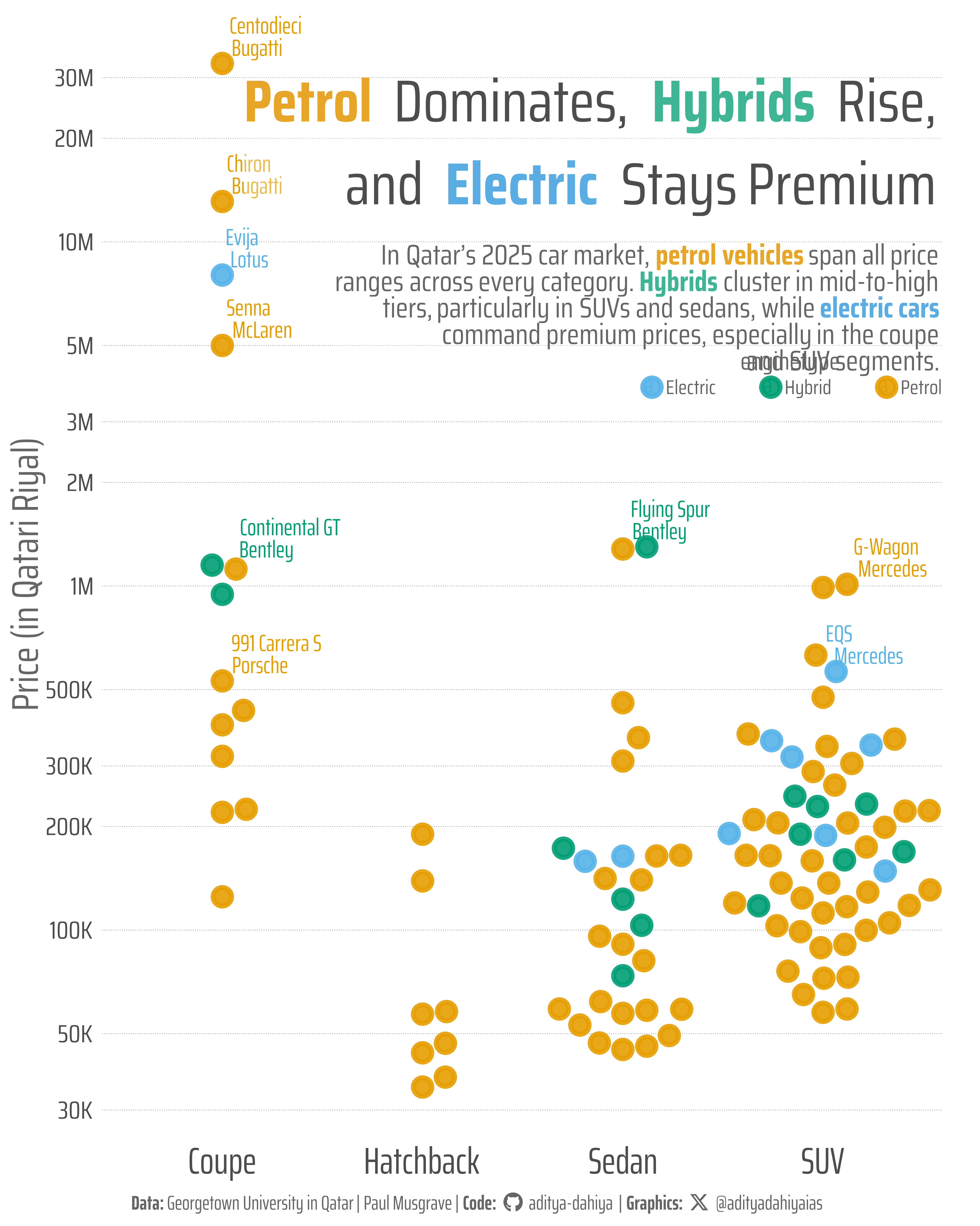
Figure 1: The graphic displays price distribution of 105 cars across four vehicle types (Coupe, Hatchback, Sedan, SUV) in Qatar’s 2025 market. Each dot represents one car, with colors indicating engine type: petrol (orange), hybrid (green), or electric (blue). The vertical axis shows prices in Qatari Riyals on a logarithmic scale, ranging from 30,000 to over 30 million QAR. The beeswarm arrangement prevents dot overlap while revealing price clustering patterns within each category.
How I Made This Graphic
.
Loading required libraries
Code
pacman::p_load( tidyverse, # All things tidy scales, # Nice Scales for ggplot2 fontawesome, # Icons display in ggplot2 ggtext, # Markdown text support for ggplot2 showtext, # Display fonts in ggplot2 colorspace, # Lighten and Darken colours patchwork # Composing Plots)pacman::p_load(ggbeeswarm)qatarcars <- readr::read_csv('https://raw.githubusercontent.com/rfordatascience/tidytuesday/main/data/2025/2025-12-09/qatarcars.csv')
Visualization Parameters
Code
# Font for titlesfont_add_google("Saira",family ="title_font")# Font for the captionfont_add_google("Saira Condensed",family ="body_font")# Font for plot textfont_add_google("Saira Extra Condensed",family ="caption_font")showtext_auto()# A base Colourbg_col <-"white"seecolor::print_color(bg_col)# Colour for highlighted texttext_hil <-"grey40"seecolor::print_color(text_hil)# Colour for the texttext_col <-"grey30"seecolor::print_color(text_col)line_col <-"grey30"# Define Base Text Sizebts <-80mypal <- paletteer::paletteer_d("ltc::trio3")[c(2, 3, 1)]# Caption stuff for the plotsysfonts::font_add(family ="Font Awesome 6 Brands",regular = here::here("docs", "Font Awesome 6 Brands-Regular-400.otf"))github <-""github_username <-"aditya-dahiya"xtwitter <-""xtwitter_username <-"@adityadahiyaias"social_caption_1 <- glue::glue("<span style='font-family:\"Font Awesome 6 Brands\";'>{github};</span> <span style='color: {text_hil}'>{github_username} </span>")social_caption_2 <- glue::glue("<span style='font-family:\"Font Awesome 6 Brands\";'>{xtwitter};</span> <span style='color: {text_hil}'>{xtwitter_username}</span>")plot_caption <-paste0("**Data:** Georgetown University in Qatar | Paul Musgrave"," | **Code:** ", social_caption_1," | **Graphics:** ", social_caption_2)rm( github, github_username, xtwitter, xtwitter_username, social_caption_1, social_caption_2)plot_title <-"<span style='color:#E8A628;'>**Petrol**</span> <span style='color:grey30;'>Dominates,</span> <span style='color:#3EB595;'>**Hybrids**</span> <span style='color:grey30;'>Rise,<br>and</span> <span style='color:#5AADE2;'>**Electric**</span> <span style='color:grey30;'>Stays Premium</span>"plot_subtitle <-"<span style='color:grey40;'>In Qatar's 2025 car market, <span style='color:#E8A628;'>**petrol vehicles**</span> span all price<br>ranges across every category. <span style='color:#3EB595;'>**Hybrids**</span> cluster in mid-to-high<br>tiers, particularly in SUVs and sedans, while <span style='color:#5AADE2;'>**electric cars**</span><br>command premium prices, especially in the coupe<br>and SUV segments.</span>"
# Saving a thumbnaillibrary(magick)# Saving a thumbnail for the webpageimage_read(here::here("data_vizs","tidy_qatar_cars.png")) |>image_resize(geometry ="x400") |>image_write( here::here("data_vizs","thumbnails","tidy_qatar_cars.png" ) )
Session Info
Code
pacman::p_load( tidyverse, # All things tidy scales, # Nice Scales for ggplot2 fontawesome, # Icons display in ggplot2 ggtext, # Markdown text support for ggplot2 showtext, # Display fonts in ggplot2 colorspace, # Lighten and Darken colours patchwork, # Composing Plots ggh4x, # Proportional facets ggchicklet, # Rounded bars ggstream # Labels in stacked bar chart)sessioninfo::session_info()$packages |>as_tibble() |># The attached column is TRUE for packages that were # explicitly loaded with library() dplyr::filter(attached ==TRUE) |> dplyr::select(package,version = loadedversion, date, source ) |> dplyr::arrange(package) |> janitor::clean_names(case ="title" ) |> gt::gt() |> gt::opt_interactive(use_search =TRUE ) |> gtExtras::gt_theme_espn()
Table 1: R Packages and their versions used in the creation of this page and graphics