LGBTQ+ Movies over the years (1990-2022)

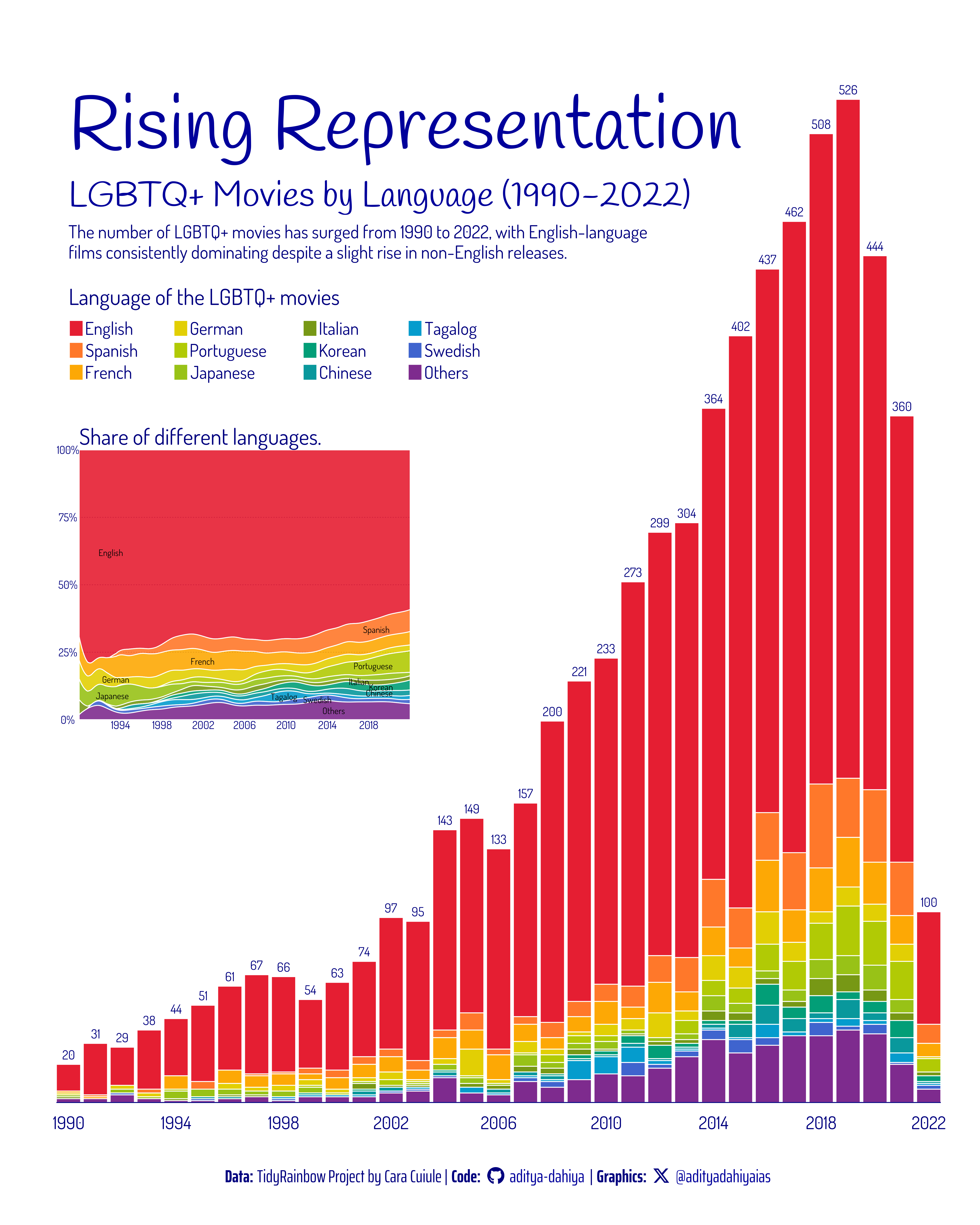
The number of LGBTQ+ movies has surged from 1990 to 2022, with English-language films consistently dominating despite a slight rise in non-English releases.

The data for this week comes from the TidyRainbow project, which is dedicated to the LGBTQ+ community using the R language ecosystem. This specific dataset, curated by Cara Cuiule, features LGBTQ+ movies. It includes comprehensive details such as movie titles, original language, release dates, popularity ratings, vote counts, and genres, among others.

The graphic displays a stacked bar graph of movie releases per year, color-coded by language, alongside a proportional stream graph showing language distribution over time. Key findings reveal a significant rise in LGBTQ+ movies, from 20 in 1990 to 526 in 2020, with English-language films dominating at around 75% of the total. While the share of non-English movies is increasing slightly, there are notable shifts such as the rise in Portuguese films and a decline in Japanese films. This indicates growing LGBTQ+ representation in cinema, though predominantly in English.

The graph illustrates the annual number of LGBTQ+ movie releases from 1990 to 2022, color-coded by language. An inset stream graph shows the proportional distribution of movie languages over the same period.

How I made this graphic?

Loading required libraries, data import & creating custom functions

# Data Import and Wrangling Tools
library(tidyverse)            # All things tidy

# Final plot tools
library(scales)               # Nice Scales for ggplot2
library(fontawesome)          # Icons display in ggplot2
library(ggtext)               # Markdown text support for ggplot2
library(showtext)             # Display fonts in ggplot2
library(colorspace)           # Lighten and Darken colours
library(patchwork)            # Combining plots

# Load data
lgbtq_movies <- readr::read_csv('https://raw.githubusercontent.com/rfordatascience/tidytuesday/master/data/2024/2024-06-25/lgbtq_movies.csv')

Exploratory Data Analysis & Data Wrangling

number_to_display = 11

# lgbtq_movies |> 
#   summarytools::dfSummary() |> 
#   summarytools::view()

df1 <- lgbtq_movies |> 
  mutate(
    year = year(release_date),
    month = month(release_date),
    day = wday(release_date, label = TRUE),
    language = original_language,
    .keep = "none"
  )

df2 <- df1 |> 
  filter(year >= 1990) |> 
  count(year, language) 

languages <- df2 |> 
  group_by(language) |> 
  summarise(n = sum(n)) |> 
  slice_max(order_by = n, n = number_to_display) |> 
  pull(language)

full_names = c("English", "Spanish", "French", "German", 
                 "Portuguese", "Japanese", "Italian", "Korean", 
                 "Chinese", "Tagalog", "Swedish", "Others")

lan_df <- tibble(
  language = c(languages, "others"),
  full_name = full_names
  )

plotdf1 <- df2 |> 
  mutate(
    language = if_else(
      language %in% languages,
      language,
      "others"
    )
  ) |> 
  group_by(year, language) |> 
  summarise(n = sum(n)) |> 
  group_by(year) |> 
  mutate(
    lang_prop = round(100*n/sum(n), 1),
    lang_prop = if_else(lang_prop > 5, lang_prop, NA)
  ) |> 
  left_join(lan_df) |> 
  mutate(
    full_name = fct(full_name, levels = full_names)
  )
 
plotdf2 <- plotdf1 |> 
  group_by(year) |> 
  summarise(total = sum(n))

Visualization Parameters

# Font for titles
font_add_google("Handlee",
  family = "title_font"
) 

# Font for the caption
font_add_google("Saira Extra Condensed",
  family = "caption_font"
) 

# Font for plot text
font_add_google("Dosis",
  family = "body_font"
) 

showtext_auto()

bg_col <- "white"
# Credits for coffeee palette
mypal <- paletteer::paletteer_d("PrettyCols::Rainbow")

text_col <-  "#00007FFF"
text_hil <-  "#00009BFF"

bts = 80

# Caption stuff for the plot
sysfonts::font_add(
  family = "Font Awesome 6 Brands",
  regular = here::here("docs", "Font Awesome 6 Brands-Regular-400.otf")
)
github <- "&#xf09b"
github_username <- "aditya-dahiya"
xtwitter <- "&#xe61b"
xtwitter_username <- "@adityadahiyaias"
social_caption_1 <- glue::glue("<span style='font-family:\"Font Awesome 6 Brands\";'>{github};</span> <span style='color: {text_hil}'>{github_username}  </span>")
social_caption_2 <- glue::glue("<span style='font-family:\"Font Awesome 6 Brands\";'>{xtwitter};</span> <span style='color: {text_hil}'>{xtwitter_username}</span>")

Annotation Text for the Plot

plot_supertitle <- "Rising Representation"

plot_title <- "LGBTQ+ Movies by Language (1990-2022)"

plot_caption <- paste0(
  "**Data:** TidyRainbow Project by Cara Cuiule", 
  " |  **Code:** ", 
  social_caption_1, 
  " |  **Graphics:** ", 
  social_caption_2
  )

plot_subtitle <- str_wrap("The number of LGBTQ+ movies has surged from 1990 to 2022, with English-language films consistently dominating despite a slight rise in non-English releases.", 80)

The static plot

g <- plotdf1 |> 
  ggplot(
    mapping = aes(
      x = year, 
      y = n
    )
  ) + 
  geom_col(
    mapping = aes(fill = full_name),
    colour = "white",
    linewidth = 0.5
  ) +
  geom_text(
    data = plotdf2,
    mapping = aes(
      y = total,
      label = total
    ),
    colour = text_col,
    nudge_y = 5,
    family = "body_font",
    size = bts / 5
  ) +
  annotate(
    geom = "text",
    label = plot_supertitle,
    x = 1990, y = 500,
    hjust = 0,
    vjust = 0,
    family = "title_font",
    size = 1.2 * bts,
    colour = text_hil
  ) +
  annotate(
    geom = "text",
    label = plot_title,
    x = 1990, y = 470,
    hjust = 0,
    vjust = 0,
    family = "title_font",
    size = bts / 1.8,
    colour = text_hil
  ) +
  annotate(
    geom = "text",
    label = plot_subtitle,
    x = 1990, y = 460,
    hjust = 0,
    vjust = 1,
    family = "body_font",
    size = bts / 3.5,
    lineheight = 0.3,
    colour = text_col
  ) +
  scale_x_continuous(
    expand = expansion(0),
    breaks = seq(1990, 2022, 4)
  ) + 
  scale_y_continuous(
    expand = expansion(c(0, 0.05))
  ) +
  scale_fill_manual(
    values = mypal
  ) +
  guides(
    fill = guide_legend(
      title = "Language of the LGBTQ+ movies",
      override.aes = list(
        pch = 20,
        size = 5
      )
    )
  ) +
  labs(
    caption = plot_caption
  ) +
  theme_classic(
    base_family = "body_font",
    base_size = bts
  ) +
  theme(
    legend.position = c(-0.025, 0.8),
    legend.justification = c(0, 1),
    legend.direction = "horizontal",
    axis.line.y = element_blank(),
    axis.ticks.length.x = unit(0, "mm"),
    axis.text.y = element_blank(),
    axis.ticks.y = element_blank(),
    axis.title = element_blank(),
    axis.text.x = element_text(
      colour = text_col
    ),
    axis.line.x = element_line(
      linewidth = 0.5,
      linetype = 1,
      colour = text_col
    ),
    axis.ticks.x = element_blank(),
    plot.caption = element_textbox(
      hjust = 0.5,
      family = "caption_font",
      colour = text_col
    ),
    legend.title = element_text(
      colour = text_col,
      lineheight = 0.3,
      hjust = 0, 
      margin = margin(0,0,5,0, "mm"),
      size = bts
    ),
    legend.title.position = "top",
    legend.text = element_text(
      colour = text_col,
      margin = margin(0,0,0,1, "mm")
    ),
    legend.key.spacing.y = unit(2, "mm"),
    legend.background = element_rect(
      fill = "transparent",
      colour = "transparent"
    )
  )

g_inset <- plotdf1 |> 
  ggplot(
    mapping = aes(
      x = year,
      y = n,
      fill = full_name,
      label = full_name
    )
  ) +
  ggstream::geom_stream(
    type = "proportional",
    colour = bg_col,
    alpha = 0.9,
    linewidth = 0.5
  ) +
  scale_x_continuous(
    expand = expansion(0),
    breaks = seq(1990, 2022, 4)
  ) +
  scale_y_continuous(
    expand = expansion(0),
    labels = label_percent()
  ) +
  coord_cartesian(clip = "off") +
  ggstream::geom_stream_label(
    type = "proportional",
    family = "body_font",
    size = bts / 7,
    hjust = "inward"
  ) +
  scale_fill_manual(
    values = mypal
  ) +
  labs(
    title = "Share of different languages."
  ) +
  theme_void(
    base_family = "body_font",
    base_size = bts / 2
  ) +
  theme(
    axis.text.y = element_text(
      colour = text_col
    ),
    axis.text.x = element_text(
      colour = text_col
    ),
    panel.grid.major.y = element_line(
      colour = text_col,
      linetype = 3
    ),
    plot.background = element_rect(
      fill = "transparent",
      colour = "transparent"
    ),
    panel.background = element_rect(
      fill = "transparent",
      colour = "transparent"
    ),
    legend.position = "none",
    plot.title = element_text(
      size = bts,
      hjust = 0,
      colour = text_col
    ), 
    plot.title.position = "panel"
  )

Plot compilation

library(patchwork)

g_full <- g + 
  inset_element(
    p = g_inset,
    left = 0, right = 0.4,
    bottom = 0.35, top = 0.65,
    align_to = "panel"
  ) +
  plot_annotation(
    theme = theme(
      plot.background = element_rect(
        fill = "transparent",
        colour = "transparent"
      ),
      panel.background = element_rect(
        fill = "transparent",
        colour = "transparent"
      )
    )
  )

Savings the graphics

ggsave(
  filename = here::here("data_vizs", "tidy_rainbow.png"),
  plot = g_full,
  width = 400,    # Best Twitter Aspect Ratio = 4:5
  height = 500,   
  units = "mm",
  bg = bg_col
)
library(magick)
# Saving a thumbnail for the webpage
image_read(here::here("data_vizs", "tidy_rainbow.png")) |> 
  image_resize(geometry = "400") |> 
  image_write(here::here("data_vizs", "thumbnails", "tidy_rainbow.png"))