Spatial analysis with {sf}, visualization with {ggplot2}, and enhanced text styling with {ggtext}
#TidyTuesday
Maps
{ggtext}
Data Wrangling
Author
Aditya Dahiya
Published
August 23, 2025
About the Data
This dataset contains information about Scottish Munros, mountains with elevations exceeding 3,000 feet (914 meters), sourced from The Database of British and Irish Hills v18.2 and made available under a Creative Commons Attribution 4.0 International Licence. Originally catalogued by Sir Hugh Munro in 1891, these peaks differ from other Scottish mountain classifications by lacking rigid prominence requirements, making the list subject to periodic revisions as new surveys are conducted. The dataset tracks the classification status of each peak across multiple revisions from 1891 to 2021, documenting whether summits were designated as full Munros, subsidiary Munro Tops, or excluded entirely during different time periods. Each entry includes precise coordinates using the British National Grid projection system, enabling geographic analysis of these iconic Scottish highlands. This data was curated by Nicola Rennie as part of the TidyTuesday weekly data project, providing researchers and enthusiasts with a comprehensive historical record of how Scotland’s most celebrated peaks have been classified over more than a century.
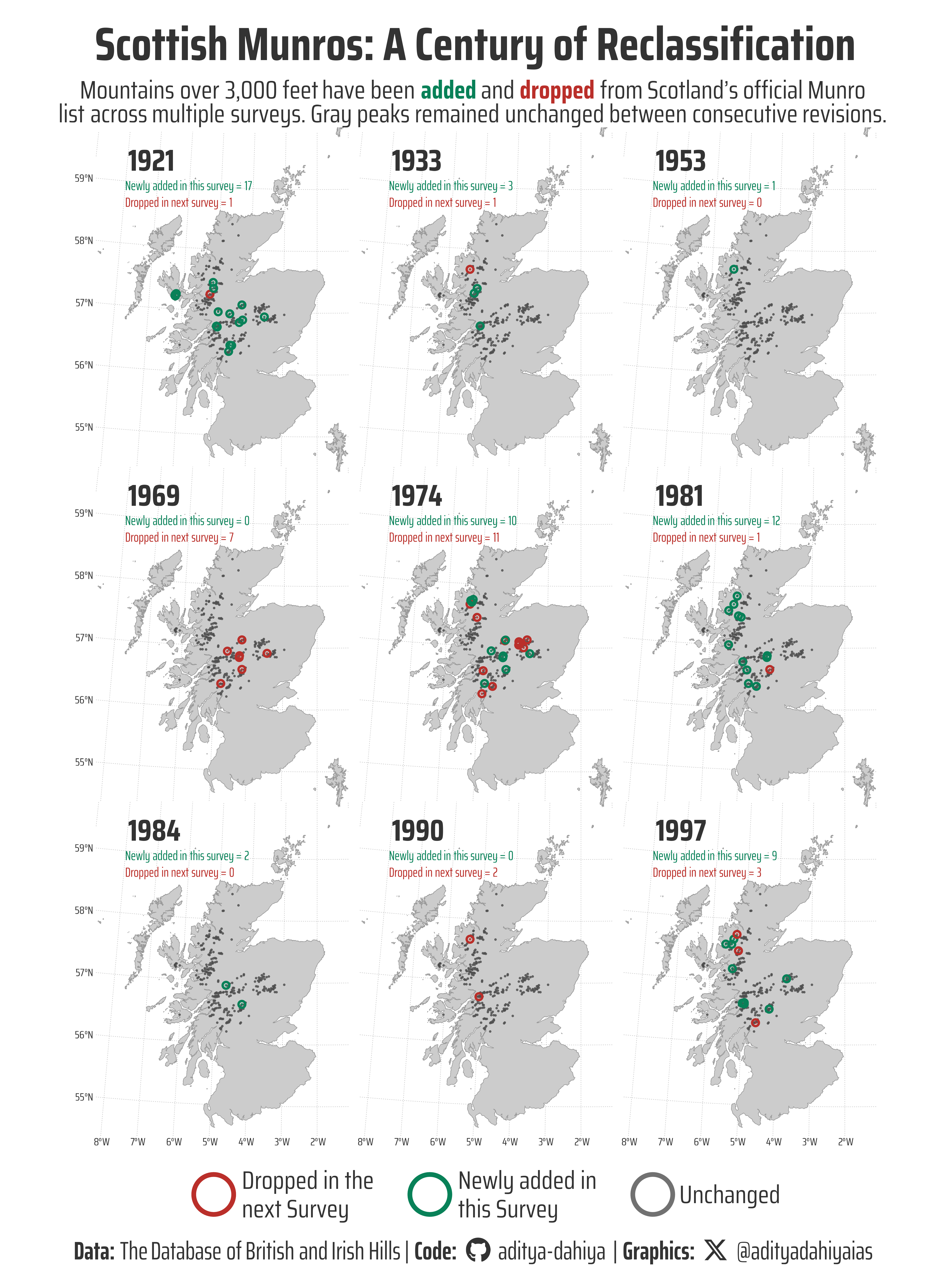
Figure 1: This map displays changes to Scotland’s official Munro list—mountains exceeding 3,000 feet in elevation—across nine survey revisions from 1921 to 1997. Each dot represents a Munro peak: green dots indicate mountains newly added to the list in that survey year, red dots show peaks that will be dropped in the next revision, and gray dots represent mountains that remained unchanged between consecutive surveys. The shifting classifications reflect improvements in surveying techniques and measurement accuracy over more than a century of Scottish mountaineering history.
How the Graphic Was Created
This visualization was created using R’s powerful mapping and data visualization ecosystem. I started by loading the Scottish Munros dataset and transforming it using the tidyverse suite of packages, particularly dplyr for data manipulation and tidyr for reshaping the data from wide to long format with pivot_longer(). The coordinate data was converted into spatial objects using the sf package’s st_as_sf() function, specifying the British National Grid (OSGB36) projection (CRS 27700). To categorize each Munro’s status across survey years, I developed custom helper functions to identify previous and next years in the chronological sequence, then used purrr’s map2_lgl() function to determine whether each peak was newly added, unchanged, or dropped in subsequent surveys. The Scotland boundary data was obtained using geodata::gadm() and transformed to match the coordinate system. The final visualization was built with ggplot2, using geom_sf() to plot both the country boundary and Munro locations, facet_wrap() to create separate panels for each survey year, and ggtext::geom_richtext() to add formatted summary statistics. Custom fonts were integrated using showtext, while the color palette and styling were enhanced with paletteer and extensive theme() customizations to create a clean, professional cartographic presentation.
Loading required libraries
Code
pacman::p_load( tidyverse, # All things tidy scales, # Nice Scales for ggplot2 fontawesome, # Icons display in ggplot2 ggtext, # Markdown text support for ggplot2 showtext, # Display fonts in ggplot2 colorspace, # Lighten and Darken colours patchwork, # Composing Plots sf)# Read in the Datascottish_munros <- readr::read_csv('https://raw.githubusercontent.com/rfordatascience/tidytuesday/main/data/2025/2025-08-19/scottish_munros.csv') |> janitor::clean_names()
Visualization Parameters
Code
# Font for titlesfont_add_google("Saira",family ="title_font") # Font for the captionfont_add_google("Saira Condensed",family ="body_font") # Font for plot textfont_add_google("Saira Extra Condensed",family ="caption_font") showtext_auto()# A base Colourbg_col <-"white"seecolor::print_color(bg_col)# Colour for highlighted texttext_hil <-"grey20"seecolor::print_color(text_hil)# Colour for the texttext_col <-"grey20"seecolor::print_color(text_col)line_col <-"grey30"# Custom Colours for dotscustom_dot_colours <- paletteer::paletteer_d("nbapalettes::cavaliers_retro")# Custom size for dotssize_var <-14# Define Base Text Sizebts <-80# Caption stuff for the plotsysfonts::font_add(family ="Font Awesome 6 Brands",regular = here::here("docs", "Font Awesome 6 Brands-Regular-400.otf"))github <-""github_username <-"aditya-dahiya"xtwitter <-""xtwitter_username <-"@adityadahiyaias"social_caption_1 <- glue::glue("<span style='font-family:\"Font Awesome 6 Brands\";'>{github};</span> <span style='color: {text_hil}'>{github_username} </span>")social_caption_2 <- glue::glue("<span style='font-family:\"Font Awesome 6 Brands\";'>{xtwitter};</span> <span style='color: {text_hil}'>{xtwitter_username}</span>")plot_caption <-paste0("**Data:** The Database of British and Irish Hills", " | **Code:** ", social_caption_1, " | **Graphics:** ", social_caption_2 )rm(github, github_username, xtwitter, xtwitter_username, social_caption_1, social_caption_2)# Add text to plot-------------------------------------------------plot_title <-"Scottish Munros: A Century of Reclassification"plot_subtitle <-"Mountains over 3,000 feet have been <span style='color:#088158FF'>**added**</span> and <span style='color:#BA2F2AFF'>**dropped**</span> from Scotland's official Munro<br>list across multiple surveys. Gray peaks remained unchanged between consecutive revisions."str_view(plot_subtitle)
Exploratory Data Analysis and Wrangling
Code
# How many distinct munors are there# scottish_munros |> # distinct(do_bih_number)# scottish_munros |> # distinct(name)# Convert into sf object for British National Grid (OSGB36) projection# df1 <- scottish_munros |> # distinct(do_bih_number, name, xcoord, ycoord, height_m) |> # drop_na() |> # st_as_sf(coords = c("xcoord", "ycoord"), crs = 27700)# # scottish_munros |> # select(height_m) |> # ggplot(aes(height_m)) +# geom_boxplot()# # df1 |> # ggplot() +# geom_sf(# aes(colour = height_m),# size = 0.8# ) +# paletteer::scale_colour_paletteer_c(# "grDevices::Purple-Yellow",# direction = -1# )df2 <- scottish_munros |>filter(!is.na(xcoord) &!is.na(ycoord)) |>st_as_sf(coords =c("xcoord", "ycoord"), crs =27700) |>st_drop_geometry() |>pivot_longer(cols =starts_with("x"),names_to ="year",values_to ="value" ) |>mutate(year =parse_number(year) ) |>filter(value =="Munro")# Code help : Clause Sonnet 4# Define the chronological order of yearsyear_order <-c(1891, 1921, 1933, 1953, 1969, 1974, 1981, 1984, 1990, 1997, 2021)# Create a helper function to get previous and next yearsget_prev_year <-function(year) { idx <-which(year_order == year)if (idx ==1) return(NA) elsereturn(year_order[idx -1])}get_next_year <-function(year) { idx <-which(year_order == year)if (idx ==length(year_order)) return(NA) elsereturn(year_order[idx +1])}# Create the label_varplotdf <- df2 |>arrange(do_bih_number, year) |>group_by(do_bih_number) |>mutate(# Get the years this munro appears inmunro_years =list(year),# For each year, check previous and nextprev_year =map_dbl(year, get_prev_year),next_year =map_dbl(year, get_next_year) ) |>ungroup() |>mutate(# Check if munro was present in previous yearwas_in_prev =case_when(is.na(prev_year) ~FALSE, # First year, so can't be continuedTRUE~map2_lgl(do_bih_number, prev_year, ~{ .x %in% (df2 |>filter(year == .y) |>pull(do_bih_number)) }) ),# Check if munro will be present in next yearwill_be_in_next =case_when(is.na(next_year) ~TRUE, # Last year, so can't be droppedTRUE~map2_lgl(do_bih_number, next_year, ~{ .x %in% (df2 |>filter(year == .y) |>pull(do_bih_number)) }) ),# Create the labellabel_var =case_when(!was_in_prev ~"Newly added in this Survey",!will_be_in_next ~"Dropped in the next Survey",TRUE~"Unchanged" ) ) |># Clean up helper columnsselect(-munro_years, -prev_year, -next_year, -was_in_prev, -will_be_in_next)plotdf1 <- plotdf |>left_join( scottish_munros |>select(do_bih_number, xcoord, ycoord) |>filter(!is.na(xcoord) &!is.na(ycoord)) |>st_as_sf(coords =c("xcoord", "ycoord"), crs =27700) ) |>st_as_sf() |>filter(!(year %in%c(1891, 2021)))# A summary table for labels in the facetplotdf2 <- plotdf |>count(year, label_var) |>pivot_wider(names_from = label_var, values_from = n, values_fill =0) |>arrange(year) |>filter(year !=1891)label_vector <-colnames(plotdf2)plotdf2 <- plotdf2 |> janitor::clean_names() |>filter(year !=2021)scotland <- geodata::gadm(country ="United Kingdom",level =1,path =tempdir(),resolution =2 ) |> janitor::clean_names() |>st_as_sf() |>filter(name_1 =="Scotland") |>st_transform(crs =27700)scotlandplotdf1plotdf2
# Saving a thumbnaillibrary(magick)# Saving a thumbnail for the webpageimage_read(here::here("data_vizs", "tidy_scottish_munros.png")) |>image_resize(geometry ="x400") |>image_write( here::here("data_vizs", "thumbnails", "tidy_scottish_munros.png" ) )
Session Info
Code
pacman::p_load( tidyverse, # All things tidy scales, # Nice Scales for ggplot2 fontawesome, # Icons display in ggplot2 ggtext, # Markdown text support for ggplot2 showtext, # Display fonts in ggplot2 colorspace, # Lighten and Darken colours patchwork # Composing Plots)sessioninfo::session_info()$packages |>as_tibble() |> dplyr::select(package, version = loadedversion, date, source) |> dplyr::arrange(package) |> janitor::clean_names(case ="title" ) |> gt::gt() |> gt::opt_interactive(use_search =TRUE ) |> gtExtras::gt_theme_espn()
Table 1: R Packages and their versions used in the creation of this page and graphics