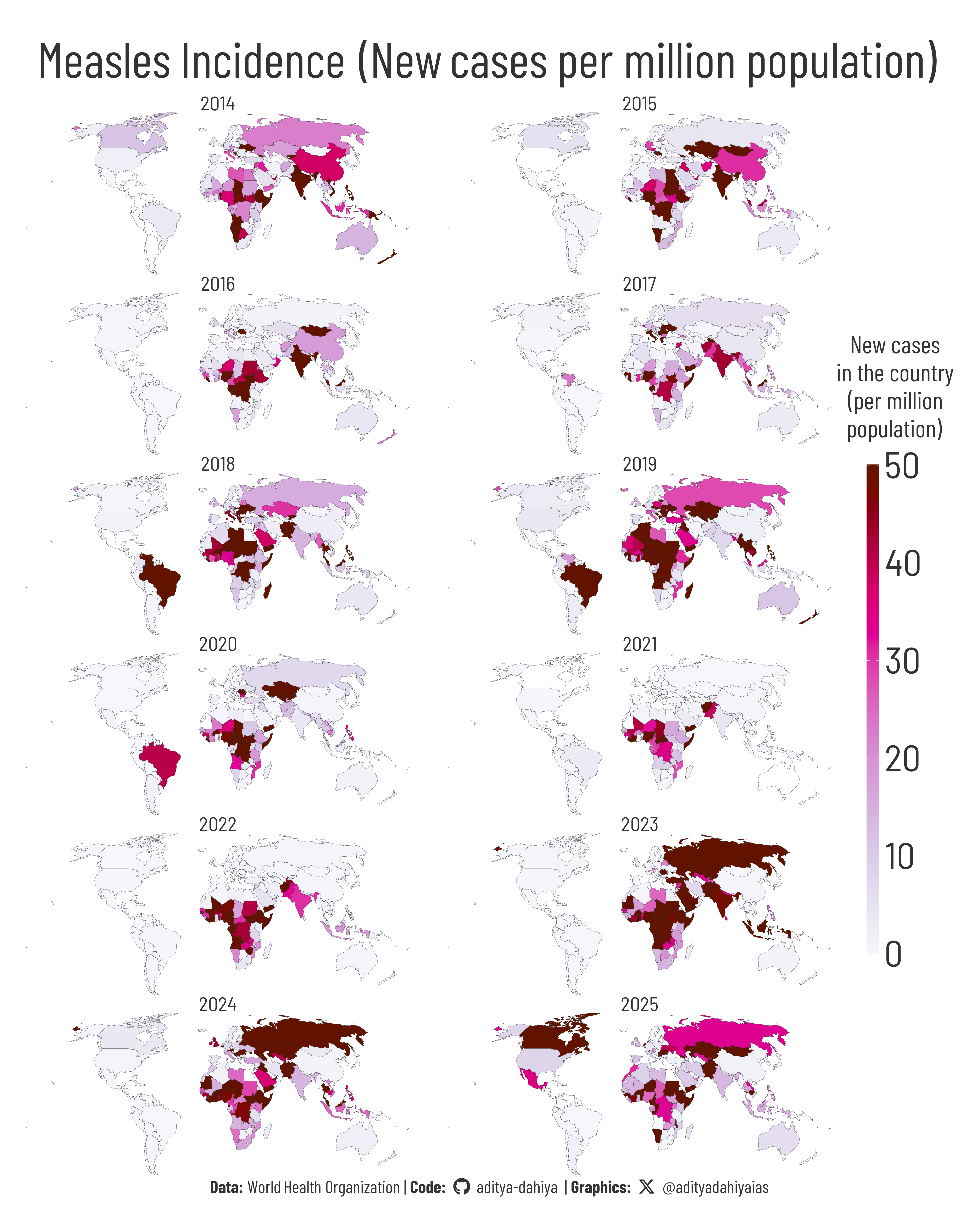
The Measles Map: Country-wise Incidence Since 2014

Facetted world map showing annual measles cases per million from 2014 to 2025 using provisional WHO data.

About the Data

This dataset presents provisional global measles and rubella case reports compiled by the World Health Organization (WHO), and was downloaded on June 12, 2025. It includes both monthly and annual figures reported by WHO Member States, covering suspected, clinically-compatible, epidemiologically-linked, and laboratory-confirmed cases. The cases_month.csv file provides monthly data by country and region, while the cases_year.csv file aggregates annual totals alongside population estimates and incidence rates. As noted by WHO, all data are provisional and subject to updates; official statistics are released each July through the WHO–UNICEF joint data collection. Users citing figures from this dataset should clearly reference the source and date, e.g., “provisional data based on monthly reports to WHO (Geneva) as of June 2025.” The data has drawn attention amid rising measles cases in the USA, but it underscores that measles remains a global threat. This week’s dataset was curated by Jen Richmond of R-Ladies Sydney for the #TidyTuesday data science community.

Figure 1: Facetted world map showing annual measles incidence (new cases per million population) from 2014 to 2025. Data are provisional and sourced from monthly WHO reports. Incidence values include suspected, confirmed, and epidemiologically linked cases as reported by Member States. Population estimates are based on WHO figures.

How the Graphic Was Created

Loading required libraries

pacman::p_load(
  tidyverse,            # All things tidy
  
  scales,               # Nice Scales for ggplot2
  fontawesome,          # Icons display in ggplot2
  ggtext,               # Markdown text support for ggplot2
  showtext,             # Display fonts in ggplot2
  colorspace,           # Lighten and Darken colours

  patchwork             # Composing Plots
)

# Option 2: Read directly from GitHub

cases_month <- readr::read_csv('https://raw.githubusercontent.com/rfordatascience/tidytuesday/main/data/2025/2025-06-24/cases_month.csv')

cases_year <- readr::read_csv('https://raw.githubusercontent.com/rfordatascience/tidytuesday/main/data/2025/2025-06-24/cases_year.csv')

Visualization Parameters

# Font for titles
font_add_google("Barlow",
  family = "title_font"
) 

# Font for the caption
font_add_google("Barlow Condensed",
  family = "caption_font"
) 

# Font for plot text
font_add_google("Barlow Semi Condensed",
  family = "body_font"
) 

showtext_auto()

# A base Colour
bg_col <- "white"
seecolor::print_color(bg_col)

# Colour for highlighted text
text_hil <- "grey20"
seecolor::print_color(text_hil)

# Colour for the text
text_col <- "grey20"
seecolor::print_color(text_col)

line_col <- "grey30"

# Define Base Text Size
bts <- 90

# Caption stuff for the plot
sysfonts::font_add(
  family = "Font Awesome 6 Brands",
  regular = here::here("docs", "Font Awesome 6 Brands-Regular-400.otf")
)
github <- "&#xf09b"
github_username <- "aditya-dahiya"
xtwitter <- "&#xe61b"
xtwitter_username <- "@adityadahiyaias"
social_caption_1 <- glue::glue("<span style='font-family:\"Font Awesome 6 Brands\";'>{github};</span> <span style='color: {text_hil}'>{github_username}  </span>")
social_caption_2 <- glue::glue("<span style='font-family:\"Font Awesome 6 Brands\";'>{xtwitter};</span> <span style='color: {text_hil}'>{xtwitter_username}</span>")
plot_caption <- paste0(
  "**Data:** World Health Organization", 
  " |  **Code:** ", 
  social_caption_1, 
  " |  **Graphics:** ", 
  social_caption_2
  )
rm(github, github_username, xtwitter, 
   xtwitter_username, social_caption_1, 
   social_caption_2)

# Add text to plot-------------------------------------------------
plot_subtitle <- str_wrap("Measles Incidence (New cases per million population)", 85)
str_view(plot_subtitle)

plot_title <- "Measles Incidence"

Exploratory Data Analysis and Wrangling

# pacman::p_load(summarytools)

# dfSummary(cases_month) |> view()

# dfSummary(cases_year) |> view()

df1 <- cases_year |> 
  select(country, iso3, year, measles_incidence_rate_per_1000000_total_population, rubella_incidence_rate_per_1000000_total_population) |> 
  rename(
    measles_incidence = measles_incidence_rate_per_1000000_total_population,
    rubella_incidence = rubella_incidence_rate_per_1000000_total_population
  ) |> 
  complete(
    iso3,
    year = 2014:2025
  ) |> 
  filter(!is.na(year))

rnaturalearth::ne_countries(returnclass = "sf") |> 
  select(iso_a3, name, geometry) |> 
  sf::st_drop_geometry() |> 
  rename(iso3 = iso_a3) |> 
  as_tibble() |> 
  distinct(iso3)

df2 <- rnaturalearth::ne_countries(returnclass = "sf") |> 
  select(iso_a3, name, geometry) |> 
  rename(iso3 = iso_a3) |> 
  filter(iso3 != "ATA")

plotdf <- df1 |> 
  left_join(df2) |> 
  sf::st_as_sf()

The Plot

g <- plotdf |> 
  filter(year >= 2014) |> 
   ggplot(
    mapping = aes(
      fill = measles_incidence,
      geometry = geometry
    )
  ) +
  geom_sf(
    linewidth = 0.1,
    colour = "grey20"
  ) +
  facet_wrap(~ year, ncol = 2) +
  coord_sf(
    crs = "ESRI:54030", 
    expand = FALSE
  ) +
  paletteer::scale_fill_paletteer_c(
    "grDevices::PuRd",
    direction = -1,
    limits = c(0, 50),
    oob = scales::squish,
    na.value = "white"
  ) +
  labs(
    # title = plot_title,
    subtitle = plot_subtitle,
    caption = plot_caption,
    fill = "New cases\nin the country\n(per million\npopulation)"
  ) +
  theme_void(
    base_family = "body_font",
    base_size = bts,
    base_line_size = bts / 100,
    base_rect_size = bts / 100
  ) +
  theme(
    # Overall
    text = element_text(
      margin = margin(0,0,0,0, "mm"),
      colour = text_col,
      lineheight = 0.3
    ),
    
    # Labels and Strip Text
    plot.subtitle = element_textbox(
      colour = text_hil,
      margin = margin(10,0,0,0, "mm"),
      size = bts * 2,
      lineheight = 0.3,
      hjust = 0.5,
      halign = 0.5,
      vjust = 0.5,
      valign = 0.5,
      family = "caption_font",
      fill = alpha("white", 0.7),
      box.color = NA,
      padding = unit(0.5, "lines"),
      r = unit(5, "mm")
    ),
    plot.caption = element_textbox(
      margin = margin(0,0,5,0, "mm"),
      hjust = 0.5,
      halign = 0.5,
      colour = text_hil,
      size = 0.7 * bts,
      family = "caption_font",
      fill = alpha("white", 0.6),
      box.color = NA,
      padding = unit(0.3, "lines"),
      r = unit(5, "mm")
    ),
    plot.caption.position = "plot",
    plot.title.position = "plot",
    plot.margin = margin(5,5,5,5, "mm"),
    panel.spacing.y = unit(0, "mm"),
    legend.position.inside = c(1, 0.5),
    legend.justification = c(1, 0.5),
    legend.direction = "vertical",
    legend.key.width = unit(5, "mm"),
    legend.key.height = unit(40, "mm"),
    legend.text.position = "right",
    legend.title.position = "top",
    legend.title = element_text(
      margin = margin(0,0,10,0, "mm"),
      hjust = 0.5,
      lineheight = 0.3,
      family = "caption_font"
    ),
    legend.text = element_text(
      margin = margin(0,0,0,3, "mm"),
      size = 1.5 * bts
    )
  )

ggsave(
  filename = here::here(
    "data_vizs",
    "tidy_usa_measles.png"
  ),
  plot = g,
  width = 400,
  height = 500,
  units = "mm",
  bg = bg_col
)

Savings the thumbnail for the webpage

# Saving a thumbnail

library(magick)

# Saving a thumbnail for the webpage
image_read(here::here("data_vizs", 
                      "tidy_usa_measles.png")) |> 
  image_resize(geometry = "x400") |> 
  image_write(
    here::here(
      "data_vizs", 
      "thumbnails", 
      "tidy_usa_measles.png"
    )
  )

Session Info

pacman::p_load(
  tidyverse,            # All things tidy
  
  scales,               # Nice Scales for ggplot2
  fontawesome,          # Icons display in ggplot2
  ggtext,               # Markdown text support for ggplot2
  showtext,             # Display fonts in ggplot2
  colorspace,           # Lighten and Darken colours

  patchwork             # Composing Plots
)


sessioninfo::session_info()$packages |> 
  as_tibble() |> 
  dplyr::select(package, 
         version = loadedversion, 
         date, source) |> 
  dplyr::arrange(package) |> 
  janitor::clean_names(
    case = "title"
  ) |> 
  gt::gt() |> 
  gt::opt_interactive(
    use_search = TRUE
  ) |> 
  gtExtras::gt_theme_espn()

Table 1: R Packages and their versions used in the creation of this page and graphics