A heatmap using {ggplot2}, {paletteer} and {ggtext}
#TidyTuesday
Author
Aditya Dahiya
Published
February 5, 2026
About the Data
The 2026 Winter Olympics dataset contains comprehensive scheduling information for all 1,866 Olympic events taking place in Milan-Cortina, Italy. Curated by Daniel Chen from Posit PBC and the University of British Columbia, this dataset is part of the weekly #TidyTuesday social data project in the R for Data Science online learning community. The data includes both competition and training sessions across various winter sport disciplines, with detailed information about start and end times in both local and UTC timezones, venue details, and metadata indicating whether events award medals. Participants can access the dataset using R with the tidytuesdayR package, Python with pandas, or Julia, and are encouraged to create visualizations, models, Quarto reports, Shiny apps, or Quarto dashboards to explore questions about event distribution, scheduling patterns, and venue utilization. The complete dataset and example code are available in the GitHub repository, by Daniel Chen.
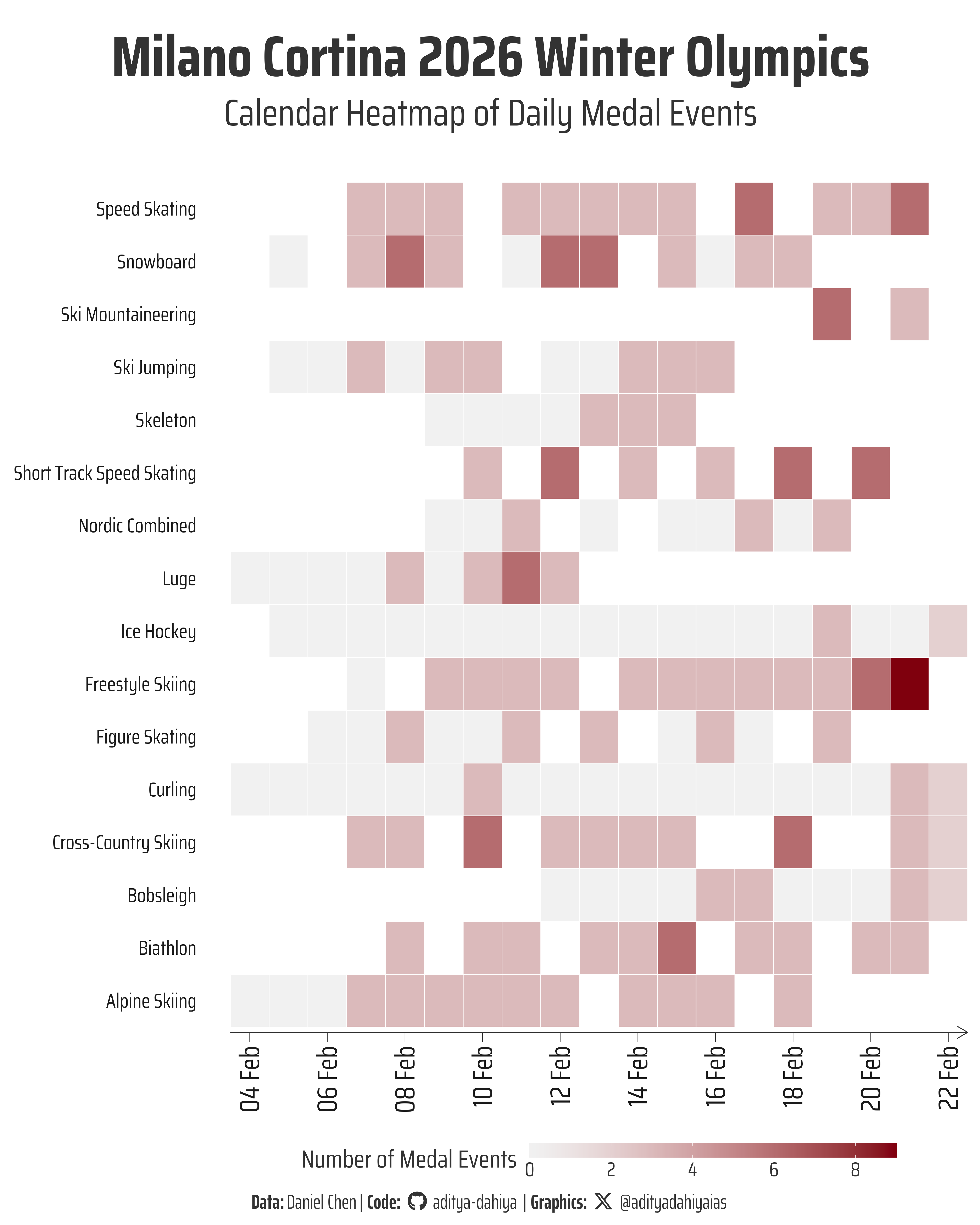
Figure 1: This calendar heatmap shows the daily distribution of medal events at the Milano Cortina 2026 Winter Olympics. Each tile represents a competition day, with deeper shades indicating a higher number of medal events. The schedule reveals how medal intensity builds across the Games, highlighting peak competition days and quieter transitions, offering a clear visual rhythm of the Olympic fortnight.
How I Made This Graphic
Loading required libraries
Code
pacman::p_load( tidyverse, # All things tidy scales, # Nice Scales for ggplot2 fontawesome, # Icons display in ggplot2 ggtext, # Markdown text support for ggplot2 showtext, # Display fonts in ggplot2 colorspace, # Lighten and Darken colours sf, # Spatial Features patchwork, # Composing Plots packcircles, # for hierarchichal packing circles colorspace, # Modify and play with colours, extract dominant colours magick # Playing with images)schedule <- readr::read_csv('https://raw.githubusercontent.com/rfordatascience/tidytuesday/main/data/2026/2026-02-10/schedule.csv')
Visualization Parameters
Code
# Font for titlesfont_add_google("Saira",family ="title_font")# Font for the captionfont_add_google("Saira Condensed",family ="body_font")# Font for plot textfont_add_google("Saira Extra Condensed",family ="caption_font")showtext_auto()# A base Colourbg_col <-"white"seecolor::print_color(bg_col)# Colour for highlighted texttext_hil <-"grey20"seecolor::print_color(text_hil)# Colour for the texttext_col <-"grey10"seecolor::print_color(text_col)# Define Base Text Sizebts <-120# Caption stuff for the plotsysfonts::font_add(family ="Font Awesome 6 Brands",regular = here::here("docs", "Font Awesome 6 Brands-Regular-400.otf"))github <-""github_username <-"aditya-dahiya"xtwitter <-""xtwitter_username <-"@adityadahiyaias"social_caption_1 <- glue::glue("<span style='font-family:\"Font Awesome 6 Brands\";'>{github};</span> <span style='color: {text_hil}'>{github_username} </span>")social_caption_2 <- glue::glue("<span style='font-family:\"Font Awesome 6 Brands\";'>{xtwitter};</span> <span style='color: {text_hil}'>{xtwitter_username}</span>")plot_caption <-paste0("**Data:** Daniel Chen"," | **Code:** ", social_caption_1," | **Graphics:** ", social_caption_2)rm( github, github_username, xtwitter, xtwitter_username, social_caption_1, social_caption_2)plot_title <-"tidy_winter_olympics"plot_subtitle <-"tidy_winter_olympics"|>str_wrap(110)
# Saving a thumbnaillibrary(magick)# Saving a thumbnail for the webpageimage_read( here::here("data_vizs","tidy_winter_olympics.png" ) ) |>image_resize(geometry ="x400") |>image_write( here::here("data_vizs","thumbnails","tidy_winter_olympics.png" ) )
Session Info
Code
pacman::p_load( tidyverse, # All things tidy scales, # Nice Scales for ggplot2 fontawesome, # Icons display in ggplot2 ggtext, # Markdown text support for ggplot2 showtext, # Display fonts in ggplot2 colorspace # Lighten and Darken colours)sessioninfo::session_info()$packages |>as_tibble() |># The attached column is TRUE for packages that were # explicitly loaded with library() dplyr::filter(attached ==TRUE) |> dplyr::select(package,version = loadedversion, date, source ) |> dplyr::arrange(package) |> janitor::clean_names(case ="title" ) |> gt::gt() |> gt::opt_interactive(use_search =TRUE ) |> gtExtras::gt_theme_espn()
Table 1: R Packages and their versions used in the creation of this page and graphics