Obesity Trajectories Across 85 Nations

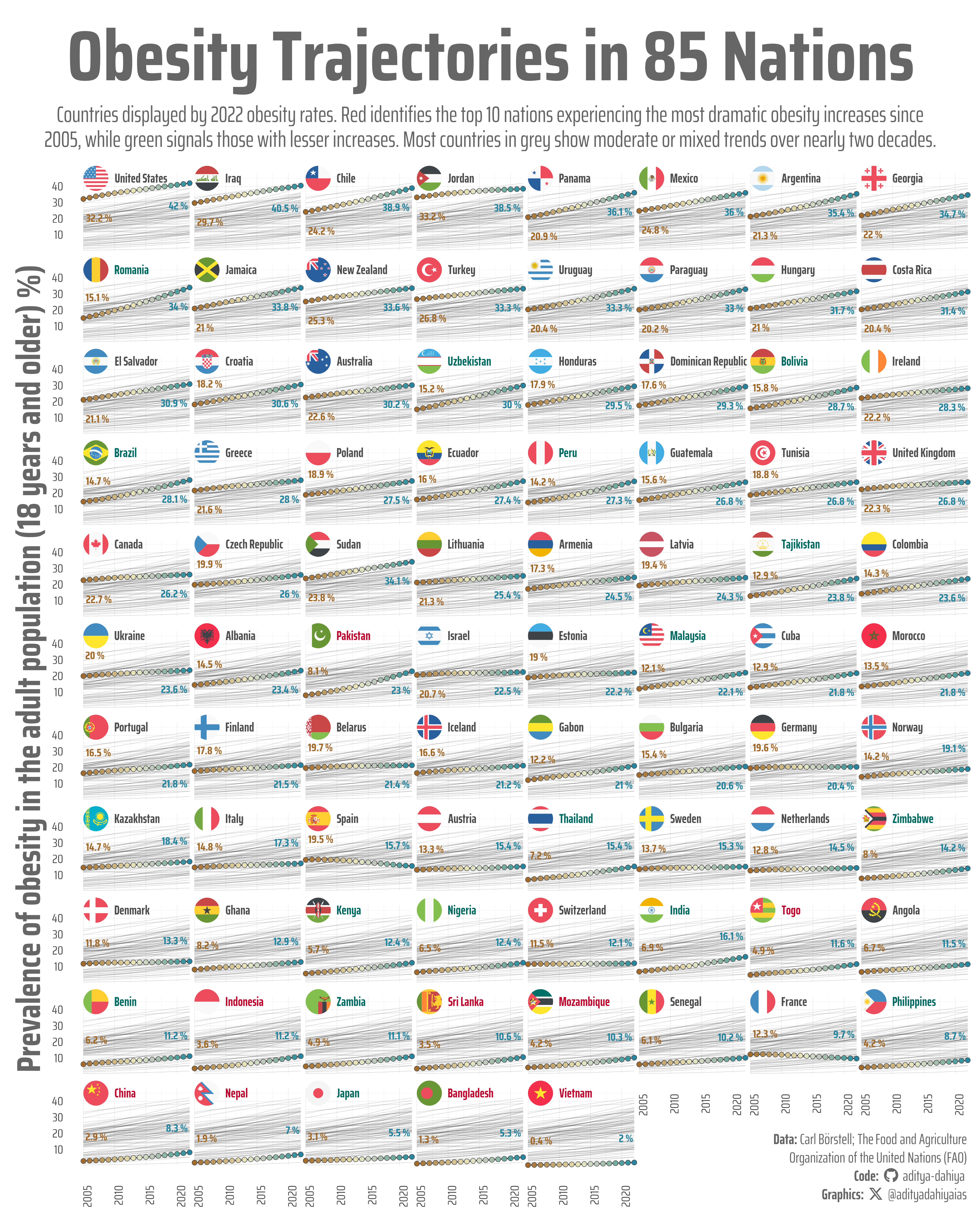
Arranged by current obesity prevalence (highest to lowest), each country’s trajectory reveals its obesity trend from 2005–2022. Red signals the top 10 fastest-rising obesity epidemics; teal indicates nations successfully reducing obesity; grey shows moderate changes.

#TidyTuesday
Facet Graph
Author

Aditya Dahiya

Published

October 20, 2025

About the Data

This week’s dataset celebrates World Food Day and the 80th anniversary of the Food and Agriculture Organization of the United Nations (FAO). The data comes from the FAO’s Suite of Food Security Indicators, a comprehensive collection developed following recommendations from the Committee on World Food Security. These indicators capture various dimensions of food insecurity using expert judgment and data with sufficient coverage to enable meaningful comparisons across regions and over time. The dataset includes measurements across multiple indicators, regions, and time periods, with confidence intervals provided for many observations to reflect measurement uncertainty. Values are expressed in diverse units including grams per capita per day, kilocalories per capita per day, international dollars, percentages, and indices, allowing for a multifaceted assessment of global food security trends.

Figure 1: Each panel represents a country, ranked by 2022 obesity rates from highest (top-left) to lowest (bottom-right). The x-axis shows years from 2005 to 2022, while the y-axis displays the prevalence of obesity in the adult population as a percentage. Lines trace each country’s trajectory over time, with values labeled at the beginning and end of the period.

How I Made This Graphic

Loading required libraries

Code
pacman::p_load(
  tidyverse, # All things tidy

  scales, # Nice Scales for ggplot2
  fontawesome, # Icons display in ggplot2
  ggtext, # Markdown text support for ggplot2
  showtext, # Display fonts in ggplot2
  colorspace, # Lighten and Darken colours
  sf, # for maps
  patchwork  # Composing Plots
)
pacman::p_load(geofacet)

food_security <- readr::read_csv('https://raw.githubusercontent.com/rfordatascience/tidytuesday/main/data/2025/2025-10-14/food_security.csv') |> 
  janitor::clean_names()

Visualization Parameters

Code
# Font for titles
font_add_google("Saira",
  family = "title_font"
)

# Font for the caption
font_add_google("Saira Condensed",
  family = "body_font"
)

# Font for plot text
font_add_google("Saira Extra Condensed",
  family = "caption_font"
)

showtext_auto()

# A base Colour
bg_col <- "white"
seecolor::print_color(bg_col)

# Colour for highlighted text
text_hil <- "grey40"
seecolor::print_color(text_hil)

# Colour for the text
text_col <- "grey30"
seecolor::print_color(text_col)

line_col <- "grey30"

# Define Base Text Size
bts <- 80

# Get the actual colors from chosen palette
day_colors <- paletteer::paletteer_d("ghibli::PonyoDark", n = 7)
names(day_colors) <- c("Sun", "Mon", "Tue", "Wed", "Thu", "Fri", "Sat")

# Caption stuff for the plot
sysfonts::font_add(
  family = "Font Awesome 6 Brands",
  regular = here::here("docs", "Font Awesome 6 Brands-Regular-400.otf")
)
github <- "&#xf09b"
github_username <- "aditya-dahiya"
xtwitter <- "&#xe61b"
xtwitter_username <- "@adityadahiyaias"
social_caption_1 <- glue::glue("<span style='font-family:\"Font Awesome 6 Brands\";'>{github};</span> <span style='color: {text_hil}'>{github_username}  </span>")
social_caption_2 <- glue::glue("<span style='font-family:\"Font Awesome 6 Brands\";'>{xtwitter};</span> <span style='color: {text_hil}'>{xtwitter_username}</span>")
plot_caption <- paste0(
  "**Data:**  Carl Börstell; The Food and Agriculture<br>Organization of the United Nations (FAO)",
  "<br>**Code:** ",
  social_caption_1,
  "<br>**Graphics:** ",
  social_caption_2
)
rm(
  github, github_username, xtwitter,
  xtwitter_username, social_caption_1,
  social_caption_2
)

# Add text to plot-------------------------------------------------
plot_title <- "Obesity Trajectories in 85 Nations"

plot_subtitle <- "Countries displayed by 2022 obesity rates. Red identifies the top 10 nations experiencing the most dramatic obesity increases since 2005, while green signals those with lesser increases. Most countries in grey show moderate or mixed trends over nearly two decades." |> 
  str_wrap(135)

str_view(plot_subtitle)

Exploratory Data Analysis and Wrangling

Code
# pacman::p_load(summarytools)
# 
# food_security |> 
#   filter(!is.na(value)) |> 
#   summarytools::dfSummary() |> 
#   summarytools::view()

# region_names <- c(
#   "Africa", "Antarctica", "Asia", "Europe", 
#   "North America", "Oceania", "South America")
# 
# food_security |> 
#   filter(area %in% region_names) |> 
#   distinct(area)

# region_names <- food_security |> 
#   distinct(area) |> 
#   slice(207:209, 211:212, 216, 218:221, 223:225, 227:229, 231:232, 237:240) |> 
#   pull(area)
# 
# region_codes <- tibble(
#   area = c(
#     "Northern America", "Northern Europe", "Caribbean", "Western Europe", 
#     "Eastern Europe", "Western Asia", "Eastern Asia", "Central Asia", 
#     "Central America", "Southern Europe", "South-eastern Asia", "Southern Asia", 
#     "South America", "Western Africa", "Northern Africa", "Eastern Africa", 
#     "Micronesia", "Middle Africa", "Southern Africa", "Australia and New Zealand", 
#     "Polynesia", "Melanesia"),
#   code = c(
#     "NA", "NE", "CB", "WE", "EE", "WA", "EA", "CA", "CM", "SE", "SA", "SIA", 
#     "SMA", "WAF", "NAF", "EAF", "MIC", "MAF", "SAF", "ANZ", "POL", "MEL"
#     )
# )
# 
# df1 <- food_security |>
#   filter(!is.na(value)) |>
#   filter(
#     item == "Prevalence of obesity in the adult population (18 years and older) (percent)"
#     ) |>
#   mutate(
#     code = countrycode::countrycode(
#       sourcevar = area,
#       origin = "country.name.en",
#       destination = "iso3c"
#     )
#   ) |>
#   filter(code %in% world_86countries_grid$code) |>
#   left_join(
#     world_86countries_grid
#   ) |>
#   select(year_start, area, code, value, name, row, col)

df1 <- food_security |> 
  filter(!is.na(value)) |> 
  filter(
    item == "Prevalence of obesity in the adult population (18 years and older) (percent)"
    ) |> 
  mutate(
    code = countrycode::countrycode(
      sourcevar = area,
      origin = "country.name.en",
      destination = "iso3c"
    )
  ) |>
  filter(code %in% world_86countries_grid$code) |> 
  left_join(
    world_86countries_grid
  ) |> 
  group_by(area) |> 
  mutate(
    value_2005 = value[year_start == 2005],
    value_2022 = value[year_start == 2022],
    pct_increase = ((value_2022 - value_2005) / value_2005) * 100
  ) |> 
  ungroup()
  
ranks_countries <- df1 |> 
  distinct(name, pct_increase) |> 
  mutate(pct_increase_rank = rank(-pct_increase, ties.method = "first"))

range(ranks_countries$pct_increase_rank)

# Identify top & bottom 10 countries by pct_increase (for colour_var)
df2 <- df1 |> 
  left_join(ranks_countries) |> 
  mutate(
    colour_var = case_when(
      pct_increase_rank <= 10 ~ "#BF092F",
      pct_increase > 77 ~ "#016B61",
      .default = "grey30"
    )
  ) |>
  mutate(
    name = fct_reorder(name, value_2022, .desc = TRUE)
  ) |> 
  group_by(name, year_start) |> 
  slice_max(n = 1, order_by = value) |> 
  ungroup() |> 
  mutate(
    country = countrycode::countrycode(
      sourcevar = name,
      origin = "country.name.en",
      destination = "iso2c"
    ),
    country = str_to_lower(country),
    vjust = case_when(
      value > 40 ~ 5,
      value > 20 ~ 4.5,
      value > 10 ~ -1,
      .default = -1.5
    )
  )

The Plot

Code
g <- df2 |> 
  ggplot(
    aes(
      y = value, 
      x = year_start
    )
  ) +
  
  # Background graphics
  geom_line(
    data = df2 |> mutate(group_var = name) |> select(-name),
    mapping = aes(group = group_var),
    linewidth = 0.2,
    alpha = 0.2
  ) +

  # Actual Geoms and Text
  geom_line(
    linewidth = 0.7,
    colour = text_col
  ) +
  geom_point(
    mapping = aes(fill = year_start),
    size = 2.5,
    pch = 21,
    stroke = 0.4,
    colour = text_col
  ) +
  paletteer::scale_fill_paletteer_c("grDevices::Earth") +
  
  geom_text(
    data = df2 |> group_by(name) |> 
            slice_max(n = 1, order_by = year_start) |> 
            ungroup(),
    mapping = aes(
      label = paste(value, "%"),
      vjust = vjust
    ),
    nudge_y = +6,
    hjust = 1.1,
    size = bts / 6,
    family = "body_font",
    fontface = "bold",
    colour = "#2686A0FF"
  ) +
  geom_text(
    data = df2 |> group_by(name) |> 
            slice_min(n = 1, order_by = year_start) |> 
            ungroup(),
    mapping = aes(
      label = paste(value, "%"),
      vjust = vjust
    ),
    nudge_y = +6,
    hjust = -0.1,
    size = bts / 6,
    family = "body_font",
    fontface = "bold",
    colour = "#A36B2BFF"
  ) +
  geom_text(
    data = df2 |> group_by(name) |> 
            slice_head(n = 1) |> ungroup(),
    mapping = aes(
      label = name,
      x = 2010,
      y = 45,
      colour = colour_var
    ),
    hjust = 0,
    vjust = 0.5,
    size = bts / 5,
    family = "caption_font",
    fontface = "bold"
  ) +
  scale_colour_identity() +
  
  # Add country flag
  ggflags::geom_flag(
    data = df2 |> group_by(name) |> 
            slice_head(n = 1) |> ungroup(),
    mapping = aes(
      country = country,
      x = 2007,
      y = 45
    ),
    size = 12
  ) +
  
  facet_wrap(
    ~name,
    ncol = 8,
    nrow = 11
    
  ) +
  # geofacet::facet_geo(
  #   grid = "world_countries_grid1",
  #   facets = ~code,
  #   move_axes = FALSE,
  #   label = "name"
  # ) +
  coord_cartesian(clip = "off") +
  scale_x_continuous(
    expand = expansion(0)
  ) +
  scale_y_continuous(
    expand = expansion(0)
  ) +
  labs(
    title = plot_title,
    subtitle = plot_subtitle,
    caption = plot_caption,
    colour = NULL,
    fill = NULL,
    x = NULL, 
    y = "Prevalence of obesity in the adult population (18 years and older) %)"
  ) +
  theme_minimal(
    base_family = "body_font",
    base_size = bts / 1.5
  ) +
  theme(
    legend.position = "none",
    
    # Overall
    text = element_text(
      margin = margin(0, 0, 0, 0, "mm"),
      colour = text_col,
      lineheight = 0.3
    ),
    
    # Grid Lines and Axes Text
    panel.grid = element_line(
      linewidth = 0.1,
      colour = alpha(text_hil, 0.3)
    ),
    axis.text.x = element_text(
      margin = margin(t = -20,r = 0,b = 0,l = 0, "mm"),
      angle = 90,
      hjust = 1
    ),
    axis.ticks = element_blank(),
    axis.ticks.length = unit(0, "mm"),
    axis.text.y = element_text(
      margin = margin(t = 0,r = -20,b = 0,l = 0, "mm")
    ),
    axis.title.x = element_blank(),
    axis.title.y = element_text(
      margin = margin(2,2,2,2, "mm"),
      colour = text_hil,
      size = bts * 1.5, 
      face = "bold"
    ),
    # Labels and Strip Text
    plot.title = element_text(
      margin = margin(5, 0, 5, 0, "mm"),
      hjust = 0.5,
      vjust = 0.5,
      colour = text_hil,
      size = 3.2 * bts,
      family = "body_font",
      face = "bold",
      lineheight = 0.25
    ),
    plot.subtitle = element_text(
      margin = margin(2, 0, 10, 0, "mm"),
      vjust = 0.5,
      colour = text_hil,
      size = bts,
      hjust = 0.5,
      family = "caption_font",
      lineheight = 0.3
    ),
    plot.caption = element_markdown(
      family = "caption_font",
      hjust = 1,
      halign = 1,
      margin = margin(-30,0,0,0, "mm"),
      colour = text_hil,
      size = bts / 1.5,
      lineheight = 0.4
    ),
    plot.caption.position = "plot",
    plot.title.position = "plot",
    plot.margin = margin(5, 5, 5, 5, "mm"),
    
    # Strip Text
    strip.text = element_blank(),
    panel.spacing.x = unit(2, "mm"),
    panel.spacing.y = unit(6, "mm")
  )

ggsave(
  filename = here::here(
    "data_vizs",
    "tidy_world_food_day.png"
  ),
  plot = g,
  width = 400,
  height = 500,
  units = "mm",
  bg = bg_col
)

Savings the thumbnail for the webpage

Code
# Saving a thumbnail

library(magick)

# Saving a thumbnail for the webpage
image_read(here::here(
  "data_vizs",
  "tidy_world_food_day.png"
)) |>
  image_resize(geometry = "x400") |>
  image_write(
    here::here(
      "data_vizs",
      "thumbnails",
      "tidy_world_food_day.png"
    )
  )

Session Info

Code
sessioninfo::session_info()$packages |>
  as_tibble() |>
  dplyr::select(package,
    version = loadedversion,
    date, source
  ) |>
  dplyr::arrange(package) |>
  janitor::clean_names(
    case = "title"
  ) |>
  gt::gt() |>
  gt::opt_interactive(
    use_search = TRUE
  ) |>
  gtExtras::gt_theme_espn()
Table 1: R Packages and their versions used in the creation of this page and graphics

Links