Colour Recognition in a Spiral

Exploring color perception through data from the xkcd Color Survey.

About the Data

The dataset comes from the xkcd Color Survey, conducted in 2010 by Randall Munroe of xkcd. In this crowdsourced experiment, hundreds of thousands of internet users were shown random colors and asked to name them. The goal was to understand how people perceive, label, and rank colors — often contradicting formal or scientific naming systems. The cleaned and structured data for the 2025-07-08 TidyTuesday challenge was curated by Nicola Rennie, and is available in three parts: answers.csv, which records users’ answers to shown hex colors; color_ranks.csv, which ranks the 954 most common RGB colors by popularity; and users.csv, containing metadata such as users’ monitor types, chromosomal sex, colorblindness status, and spam probability. The dataset provides rich opportunities to explore which users were best at naming colors, which color names appear most frequently in the top 100, and what user traits are associated with low spam probability. It is accessible via R using the tidytuesdayR package.

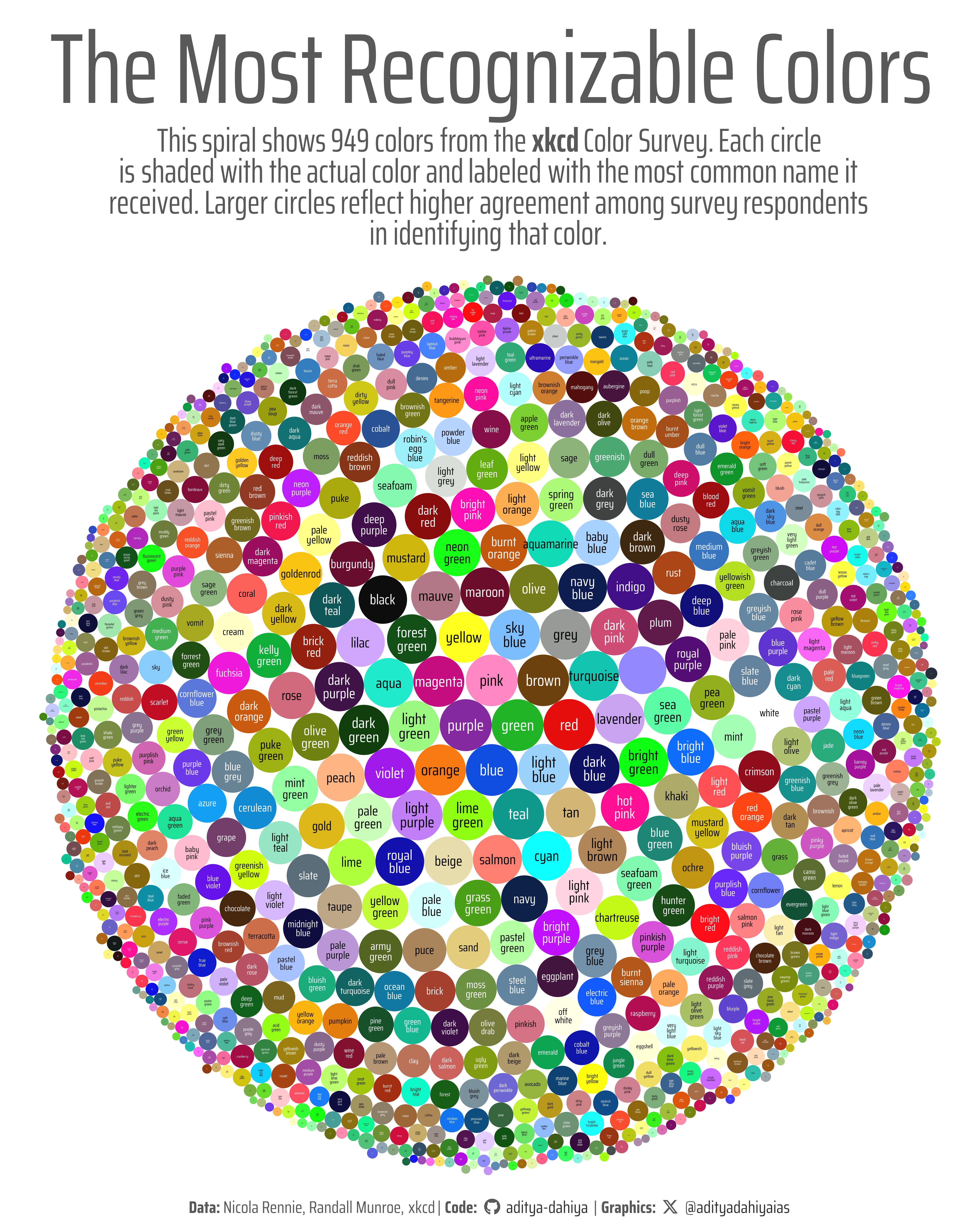
Figure 1: This spiral chart shows 949 colors from the 2010 xkcd Color Survey, where thousands of people named random colours they were shown. Each circle is filled with its actual colour and labeled with the most common name people gave it. Larger circles represent colours that were more easily and consistently recognized. The spiral layout was created using the {packcircles} and {ggplot2} packages in R, with additional tweaks for text contrast and circle sizing based on colour rank.

How the Graphic Was Created

Loading required libraries

pacman::p_load(
  tidyverse,            # All things tidy
  
  scales,               # Nice Scales for ggplot2
  fontawesome,          # Icons display in ggplot2
  ggtext,               # Markdown text support for ggplot2
  showtext,             # Display fonts in ggplot2
  colorspace,           # Lighten and Darken colours

  patchwork,            # Composing Plots
  sf                    # Making maps
)

answers <- readr::read_csv('https://raw.githubusercontent.com/rfordatascience/tidytuesday/main/data/2025/2025-07-08/answers.csv')
color_ranks <- readr::read_csv('https://raw.githubusercontent.com/rfordatascience/tidytuesday/main/data/2025/2025-07-08/color_ranks.csv')
users <- readr::read_csv('https://raw.githubusercontent.com/rfordatascience/tidytuesday/main/data/2025/2025-07-08/users.csv')

Visualization Parameters

# Font for titles
font_add_google("Saira",
  family = "title_font"
) 

# Font for the caption
font_add_google("Saira Condensed",
  family = "caption_font"
) 

# Font for plot text
font_add_google("Saira Extra Condensed",
  family = "body_font"
) 

showtext_auto()

# A base Colour
bg_col <- "white"
seecolor::print_color(bg_col)

# Colour for highlighted text
text_hil <- "grey35"
seecolor::print_color(text_hil)

# Colour for the text
text_col <- "grey20"
seecolor::print_color(text_col)

line_col <- "grey30"

# Define Base Text Size
bts <- 120

# Caption stuff for the plot
sysfonts::font_add(
  family = "Font Awesome 6 Brands",
  regular = here::here("docs", "Font Awesome 6 Brands-Regular-400.otf")
)
github <- "&#xf09b"
github_username <- "aditya-dahiya"
xtwitter <- "&#xe61b"
xtwitter_username <- "@adityadahiyaias"
social_caption_1 <- glue::glue("<span style='font-family:\"Font Awesome 6 Brands\";'>{github};</span> <span style='color: {text_hil}'>{github_username}  </span>")
social_caption_2 <- glue::glue("<span style='font-family:\"Font Awesome 6 Brands\";'>{xtwitter};</span> <span style='color: {text_hil}'>{xtwitter_username}</span>")
plot_caption <- paste0(
  "**Data:** Nicola Rennie, Randall Munroe, _xkcd_", 
  " |  **Code:** ", 
  social_caption_1, 
  " |  **Graphics:** ", 
  social_caption_2
  )
rm(github, github_username, xtwitter, 
   xtwitter_username, social_caption_1, 
   social_caption_2)

# Add text to plot-------------------------------------------------
plot_subtitle <- str_wrap(
  "This spiral shows 949 colors from the **xkcd** Color Survey. Each circle is shaded with the actual color and labeled with the most common name it received. Larger circles reflect higher agreement among survey respondents in identifying that color.",
  75) |> 
  str_replace_all("\\\n", "<br>")
str_view(plot_subtitle)

plot_title <- "The Most Recognizable Colors"

Exploratory Data Analysis and Wrangling

pacman::p_load(summarytools)

dfSummary(answers) |> view()

dfSummary(color_ranks) |> view()

dfSummary(users) |> view()

users |> 
  filter(spam_prob < 0.3) |> 
  filter(monitor == "LCD")

# answers |> 
#   left_join(color_ranks, by = join_by(hex == hex))

answers |> 
 inner_join(
    color_ranks |> 
      mutate(hex = str_to_upper(hex)),
    by = join_by(hex == hex)
  )

color_ranks |> 
  mutate(hex = str_to_upper(hex))


answers |> 
  filter(user_id == 934)

color_ranks |> 
  slice(1:10) |> 
  ggplot(aes(x = rank, y = 1, color = hex, label = color)) +
  geom_point() +
  geom_text() +
  scale_color_identity()

# Help taken from claude.ai (Sonnet 4)
# Function to determine if a hex color is dark or light
is_dark_color <- function(hex_color) {
  # Remove # if present
  hex_color <- gsub("#", "", hex_color)
  
  # Convert hex to RGB
  r <- as.numeric(paste0("0x", substr(hex_color, 1, 2)))
  g <- as.numeric(paste0("0x", substr(hex_color, 3, 4)))
  b <- as.numeric(paste0("0x", substr(hex_color, 5, 6)))
  
  # Calculate luminance using standard formula
  luminance <- (0.299 * r + 0.587 * g + 0.114 * b) / 255
  
  # Return TRUE if dark (luminance < 0.5)
  return(luminance < 0.5)
}

# Help taken from claude.ai (Sonnet 4)
# Function to get the opposite (complementary) color
get_opposite_color <- function(hex_color) {
  # Remove # if present
  hex_color <- gsub("#", "", hex_color)
  
  # Convert hex to RGB
  r <- as.numeric(paste0("0x", substr(hex_color, 1, 2)))
  g <- as.numeric(paste0("0x", substr(hex_color, 3, 4)))
  b <- as.numeric(paste0("0x", substr(hex_color, 5, 6)))
  
  # Calculate opposite RGB values (255 - original)
  r_opposite <- 255 - r
  g_opposite <- 255 - g
  b_opposite <- 255 - b
  
  # Convert back to hex
  opposite_hex <- sprintf("#%02X%02X%02X", r_opposite, g_opposite, b_opposite)
  
  return(opposite_hex)
}

# Help taken from claude.ai (Sonnet 4)
# Add spiral coordinates and exponential sizing
df1 <- color_ranks |> 
  arrange(rank)  |>
  mutate(
    # Spiral parameters
    # Adjust this value to control spiral tightness
    angle = rank * 2.4,  
    
    # Adjust multiplier to control spiral spread
    radius = sqrt(rank) * 0.3,  
    
    # Convert to x,y coordinates
    x = radius * cos(angle),
    y = radius * sin(angle),
    
    # Exponentially decreasing size
    # Adjust divisor and multiplier as needed
    size = exp(-rank/300) * 12 ,
    
    # Text color based on whether the hex color is dark or light
    text_col = ifelse(is_dark_color(hex), "white", "black"),
    
    # Opposite color for maximum contrast
    text_2_col = get_opposite_color(hex)
  )

Method 2: {packcirles}

pacman::p_load(packcircles)

##### USING {packcircles} to cerate a better spiral ######

# Create the layout using circleProgressiveLayout()
# This function returns a dataframe with a row for each bubble.
# It includes the center coordinates (x and y) and the radius, which is proportional to the value.
df1 <- color_ranks |> 
  arrange(rank)  |>
  mutate(
    # Spiral parameters
    # Adjust this value to control spiral tightness
    angle = rank * 2.4,  
    
    # Adjust multiplier to control spiral spread
    radius = sqrt(rank) * 0.3,  
    
    # Convert to x,y coordinates
    x = radius * cos(angle),
    y = radius * sin(angle),
    
    # Exponentially decreasing size
    # Adjust divisor and multiplier as needed
    size = exp(-rank/250) * 12 ,
    
    # Text color based on whether the hex color is dark or light
    text_col = ifelse(is_dark_color(hex), "white", "black"),
    
    # Opposite color for maximum contrast
    text_2_col = get_opposite_color(hex)
  )

packing1 <- circleProgressiveLayout(
  df1$size,
  sizetype = "area"
) |> 
  as_tibble()

# A tibble of centres of the circles and our cleaned data
df2 <- bind_cols(
  df1 |> 
    select(color, hex, rank, size, text_col, text_2_col),
  packing1
) |> 
  mutate(id = row_number())

# A tibble of the points on the circumference of the circles
df2_circles <- circleLayoutVertices(
  packing1,
  npoints = 100
  ) |> 
  as_tibble() |>
  mutate(id = as.numeric(id)) |> 
  
  # Adding the other variables
  left_join(
    df2 |> select(-x, -y), by = join_by(id == id)
  )

The Plot 1 (using code from Sonnet 4)

g <- df1 |> 
  ggplot(
    mapping = aes(
      x = x, y = y, 
      size = size,
      colour = hex, 
      label = str_wrap(color, width = 1) 
    )
  ) +
  geom_point() +
  geom_text(
    mapping = aes(colour = text_col),
    family = "caption_font",
    check_overlap = TRUE,
    lineheight = 0.25
  ) +
  coord_equal() +
  scale_colour_identity() +
  scale_size_identity() +
  labs(
    title = "tidy_xkcd_color_survey",
    x = NULL, y = NULL
  ) +
  theme_void(
    base_family = "body_font",
    base_size = bts
  ) +
  theme(
    legend.position = "none",
    # Overall
    text = element_text(
      margin = margin(0,0,0,0, "mm"),
      colour = text_col,
      lineheight = 0.3
    ),
    
    # Labels and Strip Text
    plot.caption = element_textbox(
      margin = margin(0,0,5,0, "mm"),
      hjust = 0.5,
      halign = 0.5,
      colour = text_hil,
      size = 0.7 * bts,
      family = "caption_font",
      fill = alpha("white", 0.6),
      box.color = NA,
      padding = unit(0.3, "lines"),
      r = unit(5, "mm")
    ),
    plot.caption.position = "plot",
    plot.title.position = "plot",
    plot.margin = margin(5,-5,5,-5, "mm")
  )

ggsave(
  filename = here::here(
    "data_vizs",
    "tidy_xkcd_color_survey.png"
  ),
  plot = g,
  width = 400,
  height = 500,
  units = "mm",
  bg = bg_col
)

The Plot 2: Using {packcircles}

g <- df2 |> 
  ggplot(
    mapping = aes(
      x = x, y = y, 
      colour = hex, 
      label = str_wrap(color, width = 1) 
    )
  ) +
  
  # Draw the packcircles
  geom_polygon(
    data = df2_circles,
    mapping = aes(
      x = x, y = y, 
      group = id,
      fill = hex,
      colour = hex
    ),
    linewidth = 0,
    alpha = 0.95
  ) +
  
  # Write the colour names
  geom_text(
    mapping = aes(
      colour = text_col,  
      size = size * 1.7
    ),
    family = "caption_font",
    check_overlap = TRUE,
    lineheight = 0.25
  ) +
  
  
  coord_equal() +
  scale_colour_identity() +
  scale_fill_identity() +
  scale_size_identity() +
  labs(
    title = plot_title,
    subtitle = plot_subtitle,
    caption = plot_caption,
    x = NULL, y = NULL
  ) +
  theme_void(
    base_family = "body_font",
    base_size = bts
  ) +
  theme(
    legend.position = "none",
    # Overall
    text = element_text(
      margin = margin(0,0,0,0, "mm"),
      colour = text_col,
      lineheight = 0.3
    ),
    
    # Labels and Strip Text
    plot.title = element_text(
      margin = margin(10,0,0,0, "mm"),
      hjust = 0.5,
      vjust = 0.5,
      colour = text_hil,
      size = 3 * bts,
      family = "body_font"
      ),
    plot.subtitle = element_textbox(
      margin = margin(5,0,-10,0, "mm"),
      hjust = 0.5,
      halign = 0.5,
      colour = text_hil,
      size = 1 * bts,
      family = "body_font",
      fill = alpha("white", 0.6),
      box.color = NA,
      padding = unit(0.3, "lines"),
      r = unit(5, "mm")
    ),
    plot.caption = element_textbox(
      margin = margin(-10,0,2,0, "mm"),
      hjust = 0.5,
      halign = 0.5,
      colour = text_hil,
      size = 0.5 * bts,
      family = "caption_font",
      fill = alpha("white", 0.6),
      box.color = NA,
      padding = unit(0.3, "lines"),
      r = unit(5, "mm")
    ),
    plot.caption.position = "plot",
    plot.title.position = "plot",
    plot.margin = margin(0,-10,0,-10, "mm")
  )

ggsave(
  filename = here::here(
    "data_vizs",
    "tidy_xkcd_color_survey.png"
  ),
  plot = g,
  width = 400,
  height = 500,
  units = "mm",
  bg = bg_col
)

Savings the thumbnail for the webpage

# Saving a thumbnail

library(magick)

# Saving a thumbnail for the webpage
image_read(here::here("data_vizs", 
                      "tidy_xkcd_color_survey.png")) |> 
  image_resize(geometry = "x400") |> 
  image_write(
    here::here(
      "data_vizs", 
      "thumbnails", 
      "tidy_xkcd_color_survey.png"
    )
  )

Session Info

pacman::p_load(
  tidyverse,            # All things tidy
  
  scales,               # Nice Scales for ggplot2
  fontawesome,          # Icons display in ggplot2
  ggtext,               # Markdown text support for ggplot2
  showtext,             # Display fonts in ggplot2
  colorspace,           # Lighten and Darken colours

  patchwork,            # Composing Plots
  packcirlcles          # To create a circle packing layout
)


sessioninfo::session_info()$packages |> 
  as_tibble() |> 
  dplyr::select(package, 
         version = loadedversion, 
         date, source) |> 
  dplyr::arrange(package) |> 
  janitor::clean_names(
    case = "title"
  ) |> 
  gt::gt() |> 
  gt::opt_interactive(
    use_search = TRUE
  ) |> 
  gtExtras::gt_theme_espn()

Table 1: R Packages and their versions used in the creation of this page and graphics