Historical Sites in the City of London (Borough of London)

A historic borough within London filled with centuries-old landmarks.

Stylized Maps with {ggmap} and {osmdata}

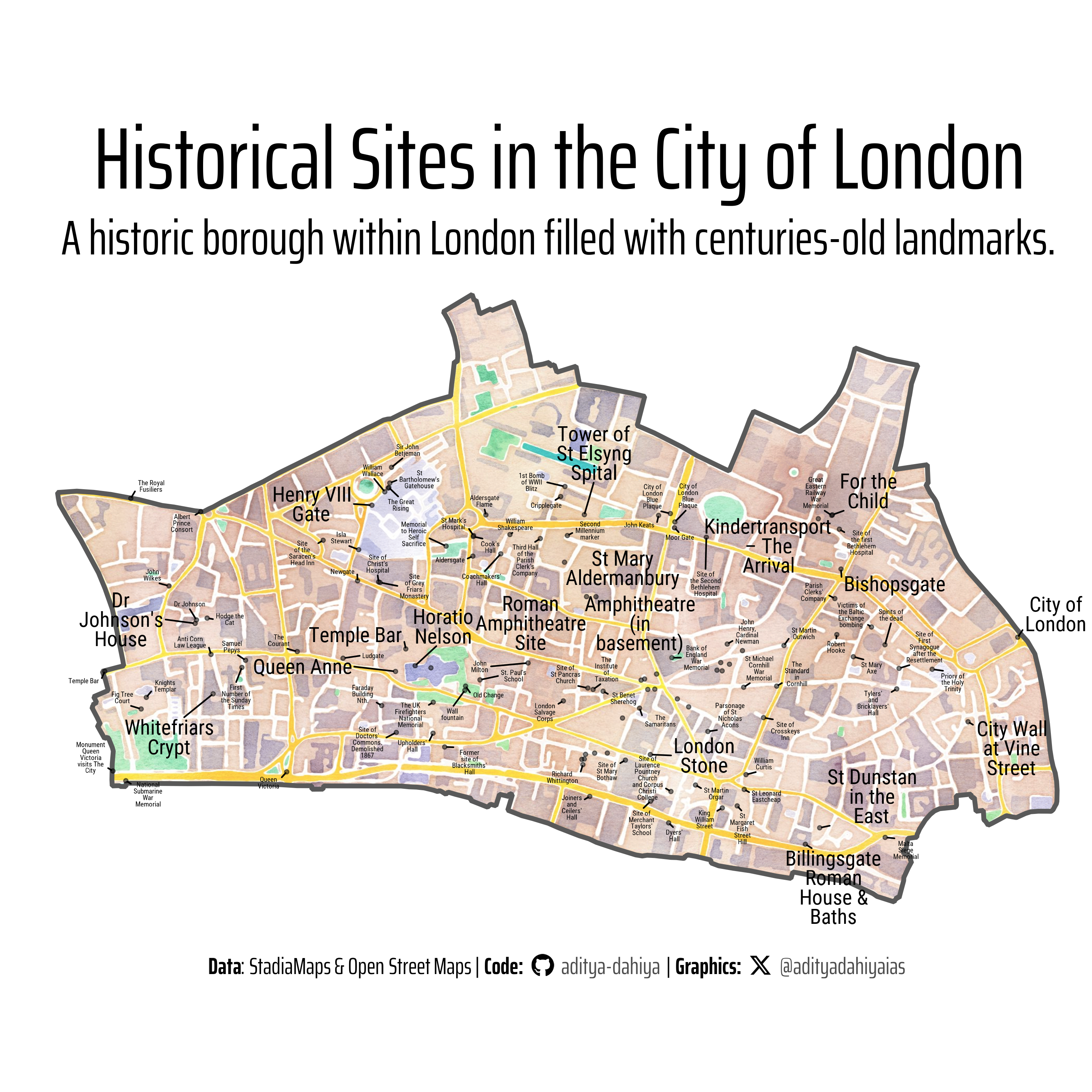
This code extracts the boundary of the City of London from the spData package and processes it using sf functions. It defines a bounding box for the area and retrieves a watercolor-style basemap from get_stadiamap(). Using osmdata, historical sites within the City of London—such as castles, memorials, and ruins—are queried from OpenStreetMap. The extracted data is filtered, transformed, and plotted with ggplot2, overlaying the historical landmarks on the base map. Labels are added using ggrepel to improve readability. The final visualization is saved using ggsave().

Loading Libraries

# Data wrangling & visualization
library(tidyverse)  # Data manipulation & visualization

# Spatial data handling
library(sf)         # Import, export, and manipulate vector data
library(terra)      # Import, export, and manipulate raster data

# ggplot2 extensions
library(tidyterra)  # Helper functions for using terra with ggplot2

# Getting raster tiles
library(ggmap)      # Getting map raster tiles
library(osmdata)    # Get Open Street Maps

# Final plot tools
library(scales)               # Nice Scales for ggplot2
library(fontawesome)          # Icons display in ggplot2
library(ggtext)               # Markdown text in ggplot2
library(showtext)             # Display fonts in ggplot2
library(patchwork)            # Composing Plots

bts = 12 # Base Text Size
sysfonts::font_add_google("Roboto Condensed", "body_font")
sysfonts::font_add_google("Oswald", "title_font")
sysfonts::font_add_google("Saira Extra Condensed", "caption_font")

showtext::showtext_auto()
# A base Colour
bg_col <- "white"
seecolor::print_color(bg_col)

# Colour for highlighted text
text_hil <- "grey30"
seecolor::print_color(text_hil)

# Colour for the text
text_col <- "grey20"
seecolor::print_color(text_col)

theme_set(
  theme_minimal(
    base_size = bts,
    base_family = "body_font"
  ) +
    theme(
      text = element_text(
        colour = "grey30",
        lineheight = 0.3,
        margin = margin(0,0,0,0, "pt")
      ),
      plot.title = element_text(
        hjust = 0.5
      ),
      plot.subtitle = element_text(
        hjust = 0.5
      )
    )
)

# Caption stuff for the plot
sysfonts::font_add(
  family = "Font Awesome 6 Brands",
  regular = here::here("docs", "Font Awesome 6 Brands-Regular-400.otf")
)
github <- "&#xf09b"
github_username <- "aditya-dahiya"
xtwitter <- "&#xe61b"
xtwitter_username <- "@adityadahiyaias"
social_caption_1 <- glue::glue("<span style='font-family:\"Font Awesome 6 Brands\";'>{github};</span> <span style='color: {text_hil}'>{github_username}  </span>")
social_caption_2 <- glue::glue("<span style='font-family:\"Font Awesome 6 Brands\";'>{xtwitter};</span> <span style='color: {text_hil}'>{xtwitter_username}</span>")
plot_caption <- paste0(
  "**Data**:  StadiaMaps & Open Street Maps",
  "  |  **Code:** ", 
  social_caption_1, 
  " |  **Graphics:** ", 
  social_caption_2
  )
rm(github, github_username, xtwitter, 
   xtwitter_username, social_caption_1, 
   social_caption_2)

city_of_london <- spData::lnd |> 
  janitor::clean_names() |> 
  filter(name == "City of London") |> 
  st_transform("EPSG:4326")

# Obtain the bounding box of London Boroughs
london_bbox <- sf::st_bbox(city_of_london)
london_bbox2 <- sf::st_bbox(city_of_london)

# A bounding box in the format c(lowerleftlon, lowerleftlat, upperrightlon, upperrightlat)
london_bbox <- c(
  left = london_bbox$xmin,
  right = london_bbox$xmax,
  bottom = london_bbox$ymin,
  top = london_bbox$ymax
)
names(london_bbox) <- c("left", "right", "bottom", "top")

# Register stadia maps API key
# register_stadiamaps("Your-Key-Here")

london_city_base <- get_stadiamap(
  bbox = london_bbox,
  zoom = 16,
  maptype = "stamen_watercolor"
)

base1 <- rast(london_city_base) |> 
  crop(city_of_london) |> 
  mask(city_of_london, touches = FALSE)

df1 <- osmdata::opq(bbox = london_bbox2) |> 
  osmdata::add_osm_feature(
    key = "historic",
    value = c("archaeological_site", "battlefield", "boundary_stone", "building", "castle", "city_gate", "citywalls", "fort", "manor", "memorial", "milestone", "monument", "ruins", "ship", "tomb", "wayside_cross", "wayside_shrine")

  ) |> 
  osmdata_sf()


df2 <- bind_rows(
  # df1$osm_multipolygons |> 
  #   filter(!is.na(name)) |> 
  #   select(name),
  
  df1$osm_polygons |> 
    filter(!is.na(name)) |> 
    select(name, historic) |> 
    st_centroid(),

  df1$osm_points |> 
    filter(!is.na(name)) |> 
    select(name, historic),
) |>
  st_transform("EPSG:4326") |> 
  st_intersection(city_of_london) |> 
  select(name, historic) |> 
  mutate(size_var = if_else(historic == "memorial", 5, 15))

df2 |> 
  st_drop_geometry() |> 
  as_tibble() |> 
  count(historic)

g <- ggplot() +
  geom_spatraster_rgb(
    data = base1,
    maxcell = Inf,
    alpha = 0.75
  ) +
  geom_sf(
    data = city_of_london,
    fill = NA,
    linewidth = 1.5,
    alpha = 0.5,
    linejoin = "bevel"
  ) +
  geom_sf(
    data = df2,
    fill =  NA,
    alpha = 0.5,
    size = 1
  ) +
  ggrepel::geom_text_repel(
    data = df2,
    mapping = aes(
      label = str_wrap(name, 10, whitespace_only = F),
      geometry = geometry,
      size = size_var
    ),
    lineheight = 0.25,
    family = "body_font",
    stat = "sf_coordinates",
    min.segment.length = unit(0, "pt"),
    force = 1,
    force_pull = 0.5,
    seed = 42,
    linewidth = 0.1
  ) +
  scale_size_identity() +
  labs(
    x = NULL, y = NULL,
    caption = plot_caption,
    title = "Historical Sites in the City of London",
    subtitle = "A historic borough within London filled with centuries-old landmarks."
  ) +
  ggthemes::theme_map(
    base_family = "body_font",
    base_size = 60
  ) +
  theme(
    plot.caption = element_textbox(
      hjust = 0.5,
      halign = 0.5,
      family = "caption_font",
      margin = margin(0,0,0,0, "pt")
    ),
    plot.title = element_text(
      margin = margin(10,0,5,0, "pt"),
      size = 180,
      family = "caption_font",
      hjust = 0.5
    ),
    plot.subtitle = element_text(
      margin = margin(5,0,0,0, "pt"),
      size = 100,
      hjust = 0.5,
      family = "caption_font"
    ),
    plot.margin = margin(0,-10,0,-10, "pt")
  )
 

ggsave(
  filename = here::here("geocomputation", 
                        "images", 
                        "ggmap_terra_3.png"),
  plot = g,
  height = 3000,
  width = 3000,
  units = "px",
  bg = "white"
)

Figure 1: Map of historical sites in the City of London, overlaid on a watercolor-style basemap. The visualization highlights key landmarks such as castles, monuments, and memorials, with point sizes indicating their type and significance.

Savings the thumbnail for the webpage

# Saving a thumbnail

library(magick)
# Saving a thumbnail for the webpage
temp <- image_read("ggmap_terra_3.png") |> 
  image_resize(geometry = "x400")
  
temp |> 
  image_write(
    here::here(
      "data_vizs", 
      "thumbnails", 
      "viz_borough_city_of_london.png"
    )
  )

Session Info

# Data wrangling & visualization
library(tidyverse)  # Data manipulation & visualization

# Spatial data handling
library(sf)         # Import, export, and manipulate vector data
library(terra)      # Import, export, and manipulate raster data

# ggplot2 extensions
library(tidyterra)  # Helper functions for using terra with ggplot2

# Getting raster tiles
library(ggmap)      # Getting map raster tiles
library(osmdata)    # Get Open Street Maps

# Final plot tools
library(scales)               # Nice Scales for ggplot2
library(fontawesome)          # Icons display in ggplot2
library(ggtext)               # Markdown text in ggplot2
library(showtext)             # Display fonts in ggplot2
library(patchwork)            # Composing Plots


sessioninfo::session_info()$packages |> 
  as_tibble() |> 
  select(package, 
         version = loadedversion, 
         date, source) |> 
  arrange(package) |> 
  janitor::clean_names(
    case = "title"
  ) |> 
  gt::gt() |> 
  gt::opt_interactive(
    use_search = TRUE
  ) |> 
  gtExtras::gt_theme_espn()

Table 1: R Packages and their versions used in the creation of this page and graphics