Postal map of Chandigarh (India) using data.gov.in

Combining {sf}, {terra}, {tidyterra} and {osmdata} to make beautiful postal code maps

About the Data

The All India Pincode Boundary GeoJSON dataset, available here, provides comprehensive geospatial information delineating postal code boundaries across India. This open data resource, published by the Government of India, includes GeoJSON files that map pincode regions with associated attributes such as pincode numbers, district names, and state names. The dataset is designed to facilitate applications in urban planning, logistics, demographic analysis, and geospatial research. Maintained under the Open Government Data (OGD) Platform India, it ensures accessibility and transparency, allowing developers, researchers, and policymakers to leverage accurate and standardized pincode-level geospatial data for various analytical and operational purposes.

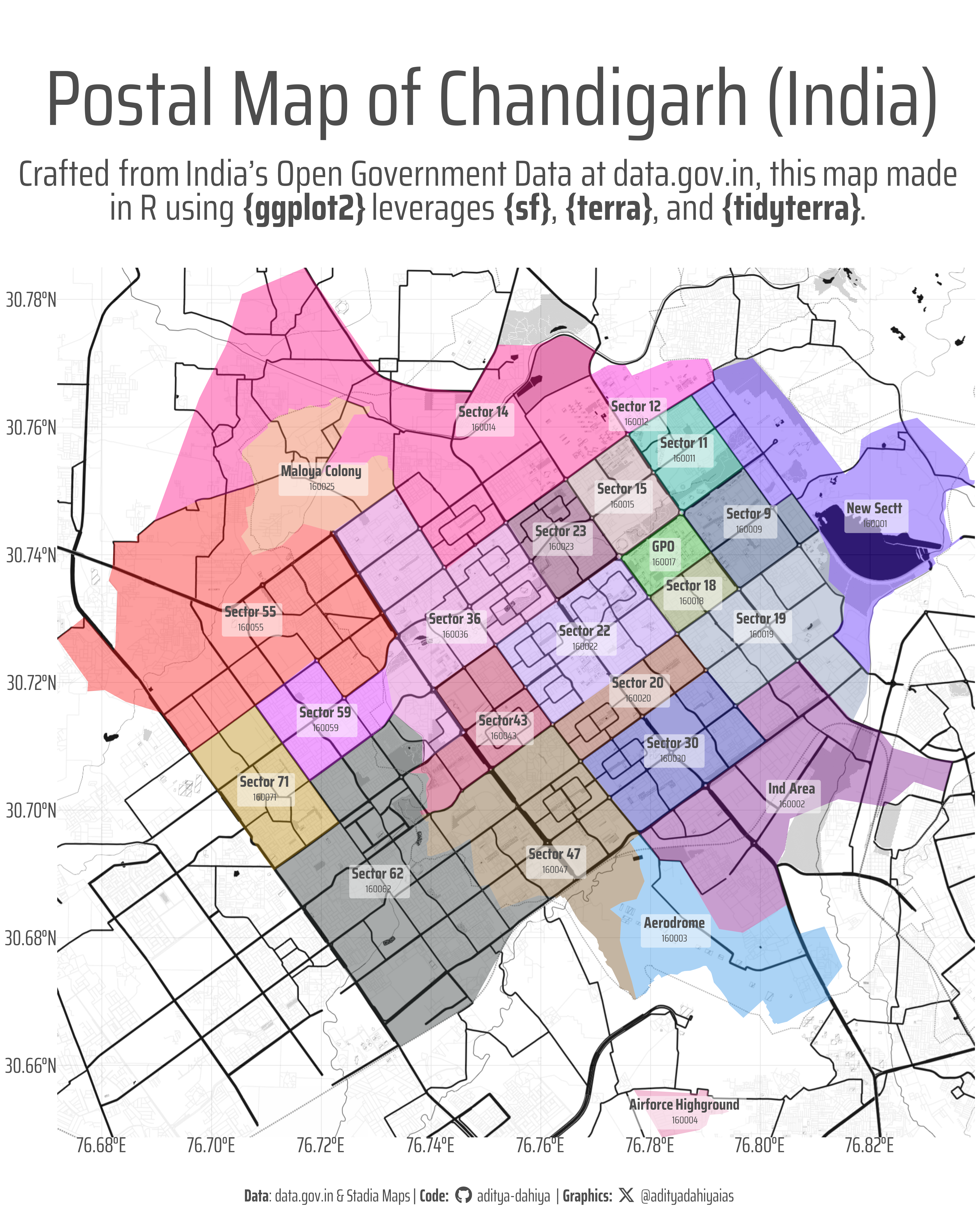
Figure 1: This map visualizes the postal zones and post office boundaries of Chandigarh, India, using open geospatial data from data.gov.in. Each zone is color-coded by post office, with labels displaying office names and pincodes, crafted with {sf}, {terra}, and {ggtext} for precision. A Stadia Maps base layer, fetched via {ggmap}, enhances context, while {ggplot2} and {tidyterra} ensure a polished output.

How I made this graphic?

This map of postal zones and post office boundaries in Chandigarh, India, was crafted using R and a suite of powerful packages for spatial data manipulation and visualization. The process started by loading key packages with pacman::p_load(), including sf for handling vector spatial data, terra for raster data support, tidyterra for integrating raster data with ggplot2, tidyverse for data wrangling, ggmap for fetching base maps, showtext for custom fonts, and ggtext for rich text labeling. I imported the All India Pincode Boundary GeoJSON data using read_sf() from the sf package, transformed it to the EPSG:4326 coordinate system with st_transform(), and filtered it to include only Chandigarh’s postal codes (160001 to 160099). A base map was retrieved from Stadia Maps via get_stadiamap(), using the bounding box of the Chandigarh postal data. The map was then built with ggplot2, layering the base map raster with geom_spatraster_rgb(), postal boundaries with geom_sf(), and post office labels with geom_richtext(). Custom fonts were applied using showtext, and the plot was polished with a minimal theme and saved as a high-resolution PNG using ggsave().

Loading required libraries

pacman::p_load(
  scales,               # Nice Scales for ggplot2
  fontawesome,          # Icons display in ggplot2
  ggtext,               # Markdown text support for ggplot2
  showtext,             # Display fonts in ggplot2
  colorspace,           # Lighten and Darken colours

  sf,                   # Maps, Simple Features in R
  terra,                # Handling Rasters
  tidyterra,            # Rasters with ggplot2
  tidyverse,            # All Data Wrangling and ggplot2
  fontawesome,          # Using fonts
  geodata,              # Get Administrative Boundaries Data
  ggmap                 # Get Base Raster Maps
)

india_pin_code <- read_sf(
  here::here(
    "data",
    "india_map",
    "All_India_pincode_Boundary-19312.geojson"
  )
) |> 
  janitor::clean_names() |> 
  st_transform("EPSG:4326") |> 
  mutate(pincode = parse_number(pincode))

haryana_map <- read_sf(
  here::here(
    "data",
    "haryana_map",
    "HARYANA_DISTRICT_BDY.shp"
  )
) |> 
  janitor::clean_names() |> 
  mutate(
    district = str_replace_all(district, ">", "A"),
    district = str_replace_all(district, "\\|", "I"),
    district = str_to_title(district)
  ) |> 
  st_transform("EPSG:4326")

haryana_outline <- read_sf(
  here::here(
    "data",
    "haryana_map",
    "HARYANA_STATE_BDY.shp"
  )
) |> 
  janitor::clean_names() |> 
  st_simplify(dTolerance = 1000) |> 
  st_transform("EPSG:4326")

chandigarh_postal <- india_pin_code |> 
  filter(pincode >= 160001 & pincode < 160100) |> 
  mutate(
    label_name = str_remove_all(office_name, "SO"),
    label_name = str_remove_all(label_name, "Chandigarh"),
    label_name = paste(
      "<b>", label_name, "</b><br><span style='font-size:30pt'>", 
      pincode,
      "</span>"
    )
  ) |> 
  relocate(label_name)


# register_stadiamap("YOUR KEY HERE")
get_map_bbox <- chandigarh_postal |> 
  st_bbox()
names(get_map_bbox) <- c("left", "bottom", "right", "top")

base_map <- get_stadiamap(
  bbox = get_map_bbox,
  zoom = 14,
  maptype = "stamen_toner_background"
) |> 
  terra::rast()

# ggplot() +
#   geom_spatraster_rgb(data = base_map)

# Get post offices in Chandigarh
# pacman::p_load(osmdata)
# 
# chandigarh_postoffices <- opq(bbox = st_bbox(chandigarh_postal)) |> 
#   add_osm_feature(
#     key = "amenity",
#     value = c("post_office", "post_box", "post_depot")
#   ) |> 
#   osmdata_sf()

Visualization Parameters

# Font for titles
font_add_google("Saira",
  family = "title_font"
) 

# Font for the caption
font_add_google("Saira Extra Condensed",
  family = "caption_font"
) 

# Font for plot text
font_add_google("Saira Condensed",
  family = "body_font"
) 

showtext_auto()

# cols4all::c4a_gui()

mypal <- paletteer::paletteer_d("NineteenEightyR::sunset2")[c(5,3,1)]

# A base Colour
bg_col <- "white"
seecolor::print_color(bg_col)

# Colour for highlighted text
text_hil <- "grey30"
seecolor::print_color(text_hil)

# Colour for the text
text_col <- "grey30"
seecolor::print_color(text_col)

line_col <- "grey30"

# Define Base Text Size
bts <- 90

# Caption stuff for the plot
sysfonts::font_add(
  family = "Font Awesome 6 Brands",
  regular = here::here("docs", "Font Awesome 6 Brands-Regular-400.otf")
)
github <- "&#xf09b"
github_username <- "aditya-dahiya"
xtwitter <- "&#xe61b"
xtwitter_username <- "@adityadahiyaias"
social_caption_1 <- glue::glue("<span style='font-family:\"Font Awesome 6 Brands\";'>{github};</span> <span style='color: {text_hil}'>{github_username}  </span>")
social_caption_2 <- glue::glue("<span style='font-family:\"Font Awesome 6 Brands\";'>{xtwitter};</span> <span style='color: {text_hil}'>{xtwitter_username}</span>")
plot_caption <- paste0(
  "**Data**:  data.gov.in & Stadia Maps",
  "  |  **Code:** ", 
  social_caption_1, 
  " |  **Graphics:** ", 
  social_caption_2
  )
rm(github, github_username, xtwitter, 
   xtwitter_username, social_caption_1, 
   social_caption_2)

Exploratory Data Analysis and Wrangling

haryana_outline |> 
  ggplot() +
  geom_sf()

haryana_map |> 
  st_drop_geometry() |> 
  select(district) |> 
  print(n = Inf)

india_pin_code |> 
  st_drop_geometry() |> 
  count(region, sort = T)
  
st_bbox(haryana_outline)

ggplot() +
  geom_sf() +
  geom_sf_text(
    aes(label = str_wrap(office_name, 5)),
    size = 2,
    lineheight = 0.7
  )

The Plot

size_var = 4000
bts = size_var / 30

# nrow(chandigarh_postal)
# cols4all::c4a_gui()
# cols4all::c4a("poly.dark24")


g <- ggplot() +
  geom_spatraster_rgb(
    data = base_map,
    maxcell = Inf,
    alpha = 0.9
  ) +
  geom_sf(
    data = chandigarh_postal,
    mapping = aes(fill = office_name),
    colour = "transparent",
    linewidth = 2,
    alpha = 0.4
  ) +
  ggtext::geom_richtext(
    data = chandigarh_postal,
    mapping = aes(
      label = label_name,
      geometry = geometry
    ),
    fill = alpha("white", 0.5),
    colour = text_col,
    lineheight = 0,
    size = bts / 8,
    hjust = 0.5, 
    vjust = 0.5,
    family = "body_font",
    stat = "sf_coordinates",
    label.size = NA,
    label.padding = unit(0.2, "lines")
  ) +
  # geom_sf(
  #   data = chandigarh_postoffices$osm_points,
  #   size = 5
  # ) +
  cols4all::scale_fill_discrete_c4a_cat("poly.dark24") +
  labs(
    x = NULL, y = NULL,
    title = "Postal Map of Chandigarh (India)",
    subtitle = "Crafted from India's Open Government Data at *data.gov.in*, this map made<br>in R using **{ggplot2}** leverages **{sf}**, **{terra}**, and **{tidyterra}**.",
    caption = plot_caption
  ) +
  coord_sf(
    crs = "EPSG:3857",
    expand = FALSE
  ) +
  theme_minimal(
    base_size = bts,
    base_family = "body_font",
    base_line_size = bts / 140,
    base_rect_size = bts / 140
  ) +
  theme(
    
    # Plot / Overall
    plot.margin = margin(5,5,5,5, "pt"),
    plot.title.position = "plot",
    plot.caption.position = "plot",
    text = element_text(
      colour = text_hil,
      lineheight = 0.3,
      margin = margin(0,0,0,0, "pt")
    ),
    
    # Plot Title, Subtitle and Caption
    plot.title = element_text(
      margin = margin(50,0,20,0, "pt"),
      hjust = 0.5,
      size = bts * 1.8
    ),
    plot.subtitle = element_textbox(
      margin = margin(0,0,40,0, "pt"),
      hjust = 0.5,
      halign = 0.5,
      size = bts / 1.2
    ),
    plot.caption = element_textbox(
      margin = margin(30,0,0,0, "pt"),
      halign = 0.5,
      hjust = 0.5,
      size = 0.4 * bts,
      family = "caption_font"
    ),
    axis.text.x = element_text(
      size = bts / 2,
      margin = margin(-0.5,0,0,0, "pt"),
      family = "caption_font"
    ),
    axis.text.y = element_text(
      size = bts / 2,
      margin = margin(0,-0.5,0,0, "pt"),
      family = "caption_font"
    ),
    axis.ticks.length = unit(0, "pt"),
    axis.ticks = element_blank(),
    
    # Legend
    legend.position = "none",
    
    # Panel
    panel.grid = element_line(
      linewidth = 0.3,
      colour = "grey0"
    )
  )


ggsave(
  plot = g,
  filename = here::here("data_vizs", 
                        "viz_chd_postal_codes.png"),
  width = size_var,
  height = (5/4) * size_var,
  units = "px",
  bg = bg_col
)

Savings the thumbnail for the webpage

# Saving a thumbnail

library(magick)

# Saving a thumbnail for the webpage
image_read(here::here("data_vizs", 
                      "viz_chd_postal_codes.png")) |> 
  image_resize(geometry = "x400") |> 
  image_write(
    here::here(
      "data_vizs", 
      "thumbnails", 
      "viz_chd_postal_codes.png"
    )
  )

Session Info

pacman::p_load(
  scales,               # Nice Scales for ggplot2
  fontawesome,          # Icons display in ggplot2
  ggtext,               # Markdown text support for ggplot2
  showtext,             # Display fonts in ggplot2
  colorspace,           # Lighten and Darken colours

  sf,                   # Maps, Simple Features in R
  terra,                # Handling Rasters
  tidyterra,            # Rasters with ggplot2
  tidyverse,            # All Data Wrangling and ggplot2
  fontawesome,          # Using fonts
  geodata,              # Get Administrative Boundaries Data
  ggmap                 # Get Base Raster Maps
)

sessioninfo::session_info()$packages |> 
  as_tibble() |> 
  dplyr::select(package, 
         version = loadedversion, 
         date, source) |> 
  dplyr::arrange(package) |> 
  janitor::clean_names(
    case = "title"
  ) |> 
  gt::gt() |> 
  gt::opt_interactive(
    use_search = TRUE
  ) |> 
  gtExtras::gt_theme_espn()

Table 1: R Packages and their versions used in the creation of this page and graphics