Customzied geographically-oriented facet with {geofacet} in R

Plotting statistics of the districts in Haryana using facet_geo() instead of facet_wrap()

About the Data

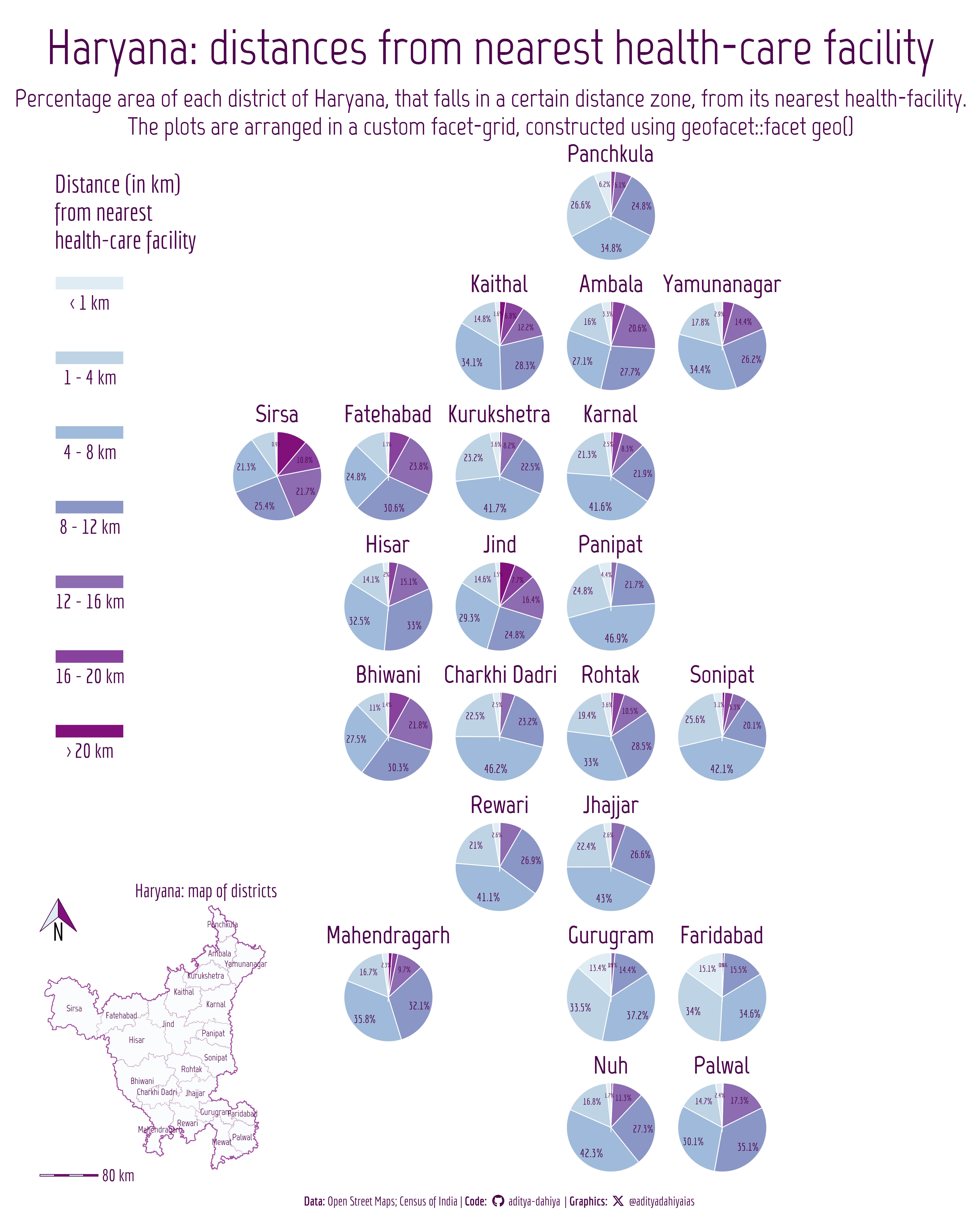
Figure 1: Pie-charts depicting the percentage area of each district of Haryana that falls within a particular distance zone from the nearest health-care facility. The charts are arranged in a customized facet pattern using geofacet::facet_geo() to mimic the approximate geographic location of the districts.

How I made this graphic?

Loading required libraries, data import & creating custom functions.

# Data Wrangling & Plotting Tools
library(tidyverse)            # All things tidy
library(sf)                   # Simple Features in R
library(geofacet)             # Geographic faceting

# Plot touch-up tools
library(scales)               # Nice Scales for ggplot2
library(fontawesome)          # Icons display in ggplot2
library(ggtext)               # Markdown text support for ggplot2
library(showtext)             # Display fonts in ggplot2
library(colorspace)           # Lighten and Darken colours
library(patchwork)            # Compiling Plots
library(tidytext)             # Getting words analysis in R

Visualization Parameters

# Font for titles
font_add_google("Marvel",
  family = "title_font"
) 

# Font for the caption
font_add_google("Economica",
  family = "caption_font"
) 

# Font for plot text
font_add_google("Economica",
  family = "body_font"
) 

showtext_auto()

mypal <- paletteer::paletteer_d("RColorBrewer::BuPu")

# A base Colour
bg_col <- mypal[1]
seecolor::print_color(bg_col)

# Colour for highlighted text
text_hil <- mypal[9]
seecolor::print_color(text_hil)

# Colour for the text
text_col <- mypal[9]
seecolor::print_color(text_col)


# Define Base Text Size
bts <- 90 

# Caption stuff for the plot
sysfonts::font_add(
  family = "Font Awesome 6 Brands",
  regular = here::here("docs", "Font Awesome 6 Brands-Regular-400.otf")
)
github <- "&#xf09b"
github_username <- "aditya-dahiya"
xtwitter <- "&#xe61b"
xtwitter_username <- "@adityadahiyaias"
social_caption_1 <- glue::glue("<span style='font-family:\"Font Awesome 6 Brands\";'>{github};</span> <span style='color: {text_hil}'>{github_username}  </span>")
social_caption_2 <- glue::glue("<span style='font-family:\"Font Awesome 6 Brands\";'>{xtwitter};</span> <span style='color: {text_hil}'>{xtwitter_username}</span>")
plot_caption <- paste0(
  "**Data:** Open Street Maps; Census of India", 
  " |  **Code:** ", 
  social_caption_1, 
  " |  **Graphics:** ", 
  social_caption_2
  )
rm(github, github_username, xtwitter, 
   xtwitter_username, social_caption_1, 
   social_caption_2)

# Add text to plot-------------------------------------------------
plot_title <- "Haryana: distances from nearest health-care facility"

plot_subtitle <- "Percentage area of each district of Haryana, that falls in a certain distance zone, from its nearest health-facility. The plots are arranged in a custom facet-grid, constructed using geofacet::facet_geo()"

Get custom data: computed using detailed R code here.

haryana_districts <- tibble(
  District_Name = c(
    "Ambala", "Bhiwani", "Charkhi Dadri", "Faridabad", "Fatehabad",
    "Gurugram", "Hisar", "Jhajjar", "Jind", "Kaithal",
    "Karnal", "Kurukshetra", "Mahendragarh", "Nuh", "Palwal",
    "Panchkula", "Panipat", "Rewari", "Rohtak", "Sirsa",
    "Sonipat", "Yamunanagar"
  ),
  Two_Letter_Code = c(
    "AM", "BH", "CD", "FR", "FT", "GU", "HI", "JH", "JI", "KT",
    "KR", "KU", "MA", "NU", "PW", "PK", "PP", "RE", "RO", "SI",
    "SN", "YN"
  ),
  Three_Letter_Code = c(
    "AMB", "BHW", "CHD", "FAR", "FAT", "GUR", "HIS", 
    "JHA", "JIN", "KAI",
    "KAR", "KUR", "MAH", "NUH", "PAL", "PAN", "PNP", 
    "REW", "ROH", "SIR", "SON", "YAM"
  ),
  Latitude = c(
    30.3782, 28.7930, 28.5921, 28.4089, 29.5252,
    28.4595, 29.1492, 28.6064, 29.3162, 29.8010,
    29.6857, 29.9695, 28.2692, 28.1070, 28.1447,
    30.6942, 29.3909, 28.1970, 28.8955, 29.5349,
    28.9931, 30.1290
  ),
  Longitude = c(
    76.7767, 76.1390, 76.2711, 77.3178, 75.4540,
    77.0266, 75.7217, 76.6565, 76.3144, 76.3995,
    76.9905, 76.8783, 76.1521, 77.0010, 77.3260,
    76.8606, 76.9635, 76.6170, 76.6066, 75.0280,
    77.0151, 77.2674
  )
)

hy_zones <- structure(list(buf_dist = structure(c(1L, 2L, 3L, 4L, 5L, 6L, 
7L, 1L, 2L, 3L, 4L, 5L, 6L, 7L, 1L, 2L, 3L, 4L, 5L, 6L, 1L, 2L, 
3L, 4L, 5L, 6L, 7L, 1L, 2L, 3L, 4L, 5L, 6L, 1L, 2L, 3L, 4L, 5L, 
6L, 7L, 1L, 2L, 3L, 4L, 5L, 6L, 1L, 2L, 3L, 4L, 5L, 6L, 7L, 1L, 
2L, 3L, 4L, 5L, 6L, 7L, 1L, 2L, 3L, 4L, 5L, 6L, 7L, 1L, 2L, 3L, 
4L, 5L, 6L, 1L, 2L, 3L, 4L, 5L, 6L, 7L, 1L, 2L, 3L, 4L, 5L, 6L, 
1L, 2L, 3L, 4L, 5L, 6L, 1L, 2L, 3L, 4L, 5L, 6L, 1L, 2L, 3L, 4L, 
5L, 6L, 1L, 2L, 3L, 4L, 5L, 6L, 1L, 2L, 3L, 4L, 5L, 6L, 7L, 1L, 
2L, 3L, 4L, 5L, 6L, 7L, 1L, 2L, 3L, 4L, 5L, 6L, 7L, 1L, 2L, 3L, 
4L, 5L, 6L, 7L, 1L, 2L, 3L, 4L, 5L, 6L), levels = c("< 1 km", 
"1 - 4 km", "4 - 8 km", "8 - 12 km", "12 - 16 km", "16 - 20 km", 
"> 20 km"), class = "factor"), district = c("Ambala", "Ambala", 
"Ambala", "Ambala", "Ambala", "Ambala", "Ambala", "Bhiwani", 
"Bhiwani", "Bhiwani", "Bhiwani", "Bhiwani", "Bhiwani", "Bhiwani", 
"Faridabad", "Faridabad", "Faridabad", "Faridabad", "Faridabad", 
"Faridabad", "Fatehabad", "Fatehabad", "Fatehabad", "Fatehabad", 
"Fatehabad", "Fatehabad", "Fatehabad", "Gurugram", "Gurugram", 
"Gurugram", "Gurugram", "Gurugram", "Gurugram", "Hisar", "Hisar", 
"Hisar", "Hisar", "Hisar", "Hisar", "Hisar", "Jhajjar", "Jhajjar", 
"Jhajjar", "Jhajjar", "Jhajjar", "Jhajjar", "Jind", "Jind", "Jind", 
"Jind", "Jind", "Jind", "Jind", "Kaithal", "Kaithal", "Kaithal", 
"Kaithal", "Kaithal", "Kaithal", "Kaithal", "Karnal", "Karnal", 
"Karnal", "Karnal", "Karnal", "Karnal", "Karnal", "Kurukshetra", 
"Kurukshetra", "Kurukshetra", "Kurukshetra", "Kurukshetra", "Kurukshetra", 
"Mahendragarh", "Mahendragarh", "Mahendragarh", "Mahendragarh", 
"Mahendragarh", "Mahendragarh", "Mahendragarh", "Mewat", "Mewat", 
"Mewat", "Mewat", "Mewat", "Mewat", "Palwal", "Palwal", "Palwal", 
"Palwal", "Palwal", "Palwal", "Panchkula", "Panchkula", "Panchkula", 
"Panchkula", "Panchkula", "Panchkula", "Panipat", "Panipat", 
"Panipat", "Panipat", "Panipat", "Panipat", "Rewari", "Rewari", 
"Rewari", "Rewari", "Rewari", "Rewari", "Rohtak", "Rohtak", "Rohtak", 
"Rohtak", "Rohtak", "Rohtak", "Rohtak", "Sirsa", "Sirsa", "Sirsa", 
"Sirsa", "Sirsa", "Sirsa", "Sirsa", "Sonipat", "Sonipat", "Sonipat", 
"Sonipat", "Sonipat", "Sonipat", "Sonipat", "Yamunanagar", "Yamunanagar", 
"Yamunanagar", "Yamunanagar", "Yamunanagar", "Yamunanagar", "Yamunanagar", 
"Charkhi Dadri", "Charkhi Dadri", "Charkhi Dadri", "Charkhi Dadri", 
"Charkhi Dadri", "Charkhi Dadri"), perc = c(0.0329, 0.1599, 0.2706, 
0.2768, 0.2065, 0.0467, 0.0066, 0.0138, 0.1099, 0.2747, 0.3029, 
0.2181, 0.0781, 0.0025, 0.1514, 0.3398, 0.3459, 0.1553, 0.0076, 
0, 0.0131, 0.1151, 0.2478, 0.3059, 0.2378, 0.0765, 0.0039, 0.134, 
0.3348, 0.3725, 0.144, 0.0148, 0, 0.0198, 0.1407, 0.3248, 0.3301, 
0.1507, 0.0327, 0.0011, 0.0263, 0.2238, 0.4302, 0.2664, 0.0528, 
5e-04, 0.0152, 0.1458, 0.2934, 0.2476, 0.1642, 0.0774, 0.0564, 
0.0164, 0.1475, 0.3411, 0.2832, 0.1225, 0.0676, 0.0218, 0.0247, 
0.2134, 0.4162, 0.219, 0.0831, 0.0358, 0.0077, 0.0358, 0.2324, 
0.4168, 0.2253, 0.0823, 0.0073, 0.0226, 0.167, 0.3579, 0.3207, 
0.0972, 0.0212, 0.0134, 0.0167, 0.1676, 0.4231, 0.2727, 0.1134, 
0.0065, 0.0242, 0.1469, 0.3006, 0.3515, 0.1731, 0.0037, 0.0618, 
0.266, 0.3477, 0.2475, 0.0607, 0.0162, 0.0445, 0.2475, 0.4688, 
0.2171, 0.0217, 4e-04, 0.0262, 0.2104, 0.4112, 0.269, 0.0819, 
0.0013, 0.0359, 0.1939, 0.3301, 0.2855, 0.1055, 0.0407, 0.0082, 
0.0088, 0.088, 0.2127, 0.2543, 0.2169, 0.1081, 0.1112, 0.0313, 
0.2556, 0.4207, 0.2006, 0.0532, 0.0293, 0.0092, 0.029, 0.1784, 
0.3443, 0.2619, 0.1442, 0.0403, 0.0019, 0.0246, 0.2249, 0.4622, 
0.2321, 0.0512, 0.005)), row.names = c(NA, -144L), class = c("tbl_df", 
"tbl", "data.frame")) |> 
  mutate(district = if_else(district == "Mewat", "Nuh", district))

# Improve hy_zones tibble into final plotting tibble "plotdf"
plotdf <- hy_zones |> 
  left_join(
    haryana_districts |> 
      select(District_Name, Three_Letter_Code),
    by = join_by(district == District_Name)
  ) |> 
  rename(code = Three_Letter_Code,
         name = district)

rm(haryana_districts, hy_zones)

Compute a custom grid using geofacet::design_grid()

haryana_grid <- data.frame(
  name = c("Panchkula", "Ambala", "Kaithal", "Yamunanagar", "Fatehabad", "Kurukshetra", "Karnal", "Sirsa", "Jind", "Panipat", "Hisar", "Rohtak", "Bhiwani", "Sonipat", "Charkhi Dadri", "Jhajjar", "Rewari", "Mahendragarh", "Faridabad", "Gurugram", "Nuh", "Palwal"),
  code = c("PAN", "AMB", "KAI", "YAM", "FAT", "KUR", "KAR", "SIR", "JIN", "PNP", "HIS", "ROH", "BHW", "SON", "CHD", "JHA", "REW", "MAH", "FAR", "GUR", "NUH", "PAL"),
  row = c(1, 2, 2, 2, 3, 3, 3, 3, 4, 4, 4, 5, 5, 5, 5, 6, 6, 7, 7, 7, 8, 8),
  col = c(4, 4, 3, 5, 2, 3, 4, 1, 3, 4, 2, 4, 2, 5, 3, 4, 3, 2, 5, 4, 4, 5),
  stringsAsFactors = FALSE
)

The Base Plot

g <- plotdf |> 
  ggplot(
    mapping = aes(
      x = 1,
      y = perc,
      group = buf_dist,
      fill = buf_dist
    )
  ) +
  geom_col(
    position = position_stack(),
    colour = "white",
    linewidth = 0.5
  ) +
  geom_text(
    mapping = aes(
      label = paste0(round(100 * perc, 1), "%"),
      x = 1.2,
      size = perc
    ),
    position = position_stack(
      vjust = 0.5
    ),
    family = "body_font",
    check_overlap = TRUE,
    colour = text_col
  ) +
  scale_size(range = c(bts/15, bts/6)) +
  scale_x_continuous(expand = expansion(0)) +
  scale_fill_manual(
    values = mypal[2:8]
  ) +
  facet_geo(
    ~code, 
    grid = haryana_grid,
    label = "name"
  ) +
  coord_radial(
    theta = "y",
    expand = FALSE,
    clip = "off"
  ) +
  guides(size = "none") +
  labs(
    x = NULL, y = NULL,
    fill = "Distance (in km)\nfrom nearest \nhealth-care facility",
    title = plot_title,
    subtitle = plot_subtitle |> str_wrap(120),
    caption = plot_caption
  ) +
  theme_minimal(
    base_family = "body_font",
    base_size = bts
  ) +
  theme(
    # Full plot features
    plot.margin = margin(10,10,5,10, "mm"),
    panel.grid = element_blank(),
    axis.text = element_blank(),
    plot.title.position = "plot",
    text = element_text(
      colour = text_col
    ),
    # Legend
    legend.position = "inside",
    legend.position.inside = c(-0.3,1),
    legend.justification = c(0,1),
    legend.direction = "vertical",
    legend.box = "vertical",
    legend.box.spacing = unit(0, "mm"),
    legend.margin = margin(0,0,0,0, "mm"),
    legend.box.margin = margin(0,0,0,0, "mm"),
    legend.text = element_text(
      margin = margin(2,0,15,0, "mm"),
      colour = text_col
    ),
    legend.title = element_text(
      margin = margin(5,0,10,0, "mm"),
      colour = text_col,
      hjust = 0,
      lineheight = 0.3
    ),
    legend.title.position = "top",
    legend.key.height = unit(6, "mm"),
    legend.key.width = unit(5, "mm"),
    legend.text.position = "bottom",
    legend.location = "plot",
    
    
    
    # Strip Texts
    strip.text = element_text(
      margin = margin(0,0,-2,0, "mm"),
      size = bts,
      family = "title_font",
      colour = text_col,
      hjust = 0.5,
      face = "bold"
    ),
    panel.spacing = unit(0, "mm"),
    
    # Labels and titles
    plot.title = element_text(
      hjust = 0.5,
      size = 2 * bts,
      family = "title_font",
      lineheight = 0.3,
      margin = margin(0,0,5,0, "mm")
    ),
    plot.subtitle = element_text(
      hjust = 0.5,
      size = bts,
      family = "title_font",
      lineheight = 0.3,
      margin = margin(0,0,0,0, "mm")
    ),
    plot.caption = element_textbox(
      hjust = 0.5,
      family = "caption_font",
      lineheight = 0.3,
      margin = margin(5,0,0,0, "mm"),
      size = 0.5 * bts
    )
  )

Inset Plot: Map of Haryana

region_map <- sf::read_sf(
  here::here("data", "india_map", "India_State_Boundary.shp")
) |> 
  janitor::clean_names() |> 
  filter(state_name == "Haryana")

districts_map <- sf::read_sf(
  here::here("data", "haryana_map", "HARYANA_DISTRICT_BDY.shp")
) |> 
  janitor::clean_names() |> 
  select(district, state, shape_leng, shape_area, geometry) |> 
  mutate(
    state = str_replace_all(state, ">", "A"),
    district = str_replace_all(district, ">", "A"),
    district = str_replace_all(district, "\\|", "I"),
    district = str_to_title(district)
  )


g_inset <- ggplot() +
  
  geom_sf(
    data = districts_map,
    colour = mypal[8],
    linewidth = 0.2,
    linetype = 3,
    fill = alpha(mypal[4], 0.05)
  ) +
  geom_sf_text(
    data = districts_map,
    mapping = aes(label = district),
    colour = text_col,
    family = "title_font",
    size = bts / 8
  ) +
  
  geom_sf(
    data = region_map,
    colour = alpha(mypal[8], 0.7),
    linewidth = 0.5,
    fill = NA
  ) +
  # Add North-Arrow and Scale
  ggspatial::annotation_north_arrow(
    style = ggspatial::north_arrow_orienteering(
      line_col = text_col,
      fill = c(mypal[2], mypal[8]),
      text_size = bts,
      text_family = "body_font"
    ),
    location = "tl",
    height = unit(15, "mm"),
    width = unit(15, "mm")
  ) +
  ggspatial::annotation_scale(
    bar_cols = c(mypal[2], mypal[8]),
    location = "bl",
    line_col = text_col,
    height = unit(0.75, "mm"),
    text_cex = 5,
    text_family = "body_font",
    text_col = text_col
  ) +
  labs(
    title = "Haryana: map of districts" 
  ) +
  ggthemes::theme_map(
    base_size = bts / 2,
    base_family = "body_font"
  ) +
  theme(
    plot.title = element_text(
      colour = text_col,
      margin = margin(0,0,-10,0),
      hjust = 1,
      size = bts * 0.75
    )
  )

Compile plot

g_final <- g +
  inset_element(
    p = g_inset,
    left = 0, right = 0.3,
    bottom = 0, top = 0.3,
    align_to = "full",
    clip = FALSE
  )

ggsave(
  filename = here::here(
    "data_vizs",
    "viz_custom_facet_hy.png"
  ),
  plot = g_final,
  width = 400,
  height = 500,
  units = "mm",
  bg = bg_col
)

Savings the thumbnail for the webpage

# Saving a thumbnail

library(magick)
# Saving a thumbnail for the webpage
image_read(here::here("data_vizs", 
                      "viz_custom_facet_hy.png")) |> 
  image_resize(geometry = "x400") |> 
  image_write(
    here::here(
      "data_vizs", 
      "thumbnails", 
      "viz_custom_facet_hy.png"
    )
  )

Session Info

# Data Wrangling & Plotting Tools
library(tidyverse)            # All things tidy
library(sf)                   # Simple Features in R
library(geofacet)             # Geographic faceting

# Plot touch-up tools
library(scales)               # Nice Scales for ggplot2
library(fontawesome)          # Icons display in ggplot2
library(ggtext)               # Markdown text support for ggplot2
library(showtext)             # Display fonts in ggplot2
library(colorspace)           # Lighten and Darken colours
library(patchwork)            # Compiling Plots
library(tidytext)             # Getting words analysis in R

sessioninfo::session_info()$packages |> 
  as_tibble() |> 
  select(package, 
         version = loadedversion, 
         date, source) |> 
  arrange(package) |> 
  janitor::clean_names(
    case = "title"
  ) |> 
  gt::gt() |> 
  gt::opt_interactive(
    use_search = TRUE
  ) |> 
  gtExtras::gt_theme_espn()

Table 1: R Packages and their versions used in the creation of this page and graphics