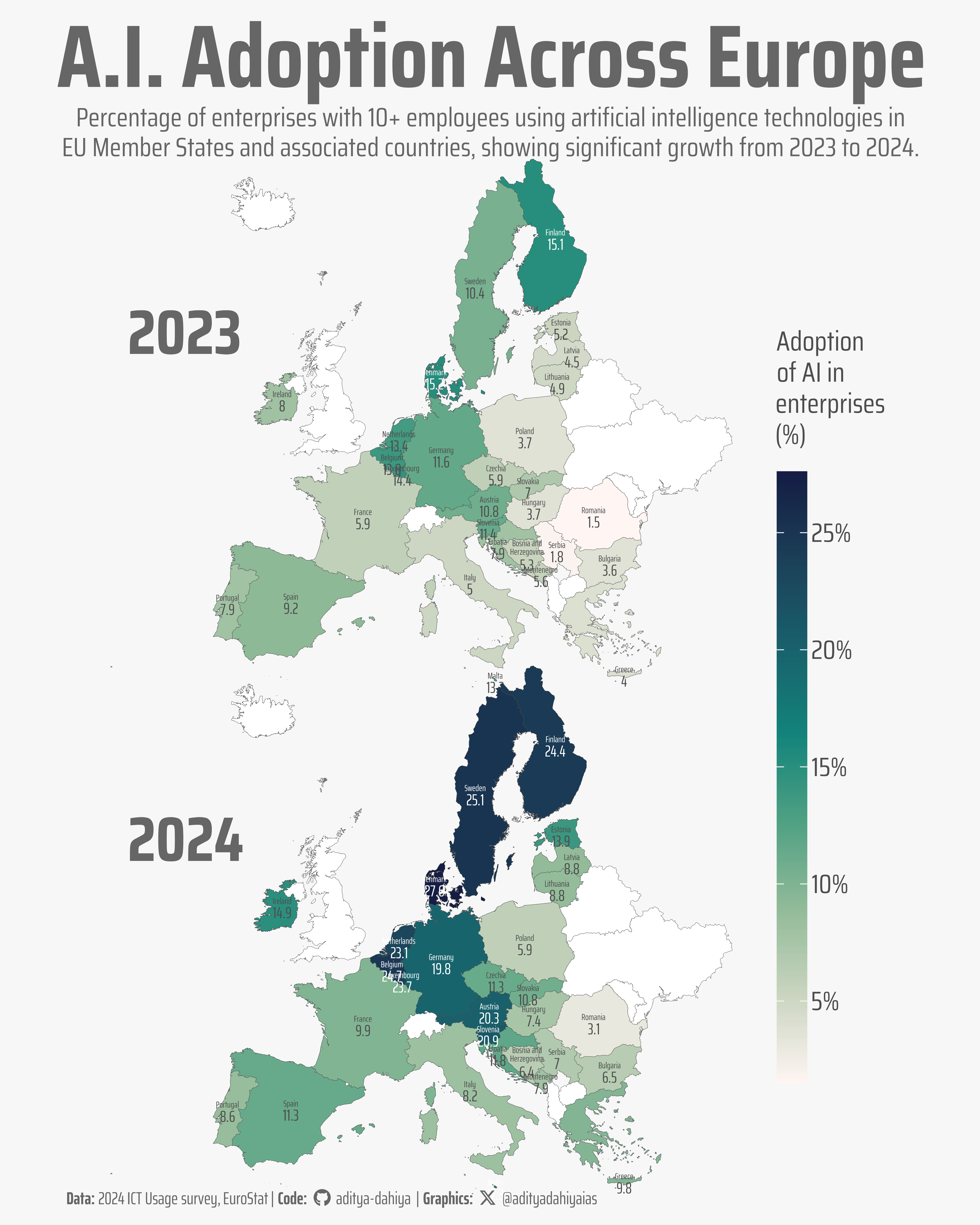
Share of businesses adopting AI technologies including text mining, machine learning, and natural language processing across European nations, with Denmark, Sweden, and Belgium leading adoption rates.
Chloropleth
Maps
Author
Aditya Dahiya
Published
August 26, 2025
About the Data
The data presented in this visualization comes from Eurostat’s 2024 EU survey on ‘ICT usage and e-commerce in enterprises’, conducted by National Statistical Authorities in the first months of 2024. The survey reveals that 13.5% of enterprises in the EU with 10 or more employees used artificial intelligence (AI) technologies to conduct their business in 2024, representing a significant 5.5 percentage point growth from 8.0% in 2023. The comprehensive survey covered approximately 157,000 of the 1.54 million enterprises across the EU, with data collection focusing on enterprises with at least 10 employees and self-employed persons across multiple economic sectors including manufacturing, information and communication, professional services, and retail trade. AI technologies measured in the survey include text mining, speech recognition, natural language generation, image recognition, machine learning, robotic process automation, and autonomous decision-making systems. The original data and detailed methodology are available through Eurostat’s database, with the specific Excel file containing the visualization data accessible at the European Commission’s statistics portal.
Figure 1: This map visualizes the percentage of enterprises with 10 or more employees using artificial intelligence technologies across European countries in 2023 and 2024. The fill colors represent AI adoption rates, ranging from light (low adoption) to dark (high adoption), with values displayed on each country. Denmark leads with 27.6% adoption in 2024, followed by Sweden (25.1%) and Belgium (24.7%), while Romania shows the lowest rate at 3.1%. All countries demonstrate growth between the two years, reflecting Europe’s accelerating digital transformation. Data source: Eurostat’s ICT usage survey.
How I Made This Graphic
This visualization was created using R and several key packages for data processing, spatial analysis, and plotting. The data was harvested directly from Eurostat’s Excel file using R’s built-in download.file() function and processed with the readxl package to extract specific sheet ranges. Data wrangling was performed using the tidyverse ecosystem, particularly dplyr for data manipulation and tidyr for reshaping the data from wide to long format. Country names were standardized and converted to ISO3 codes using the countrycode package. The spatial component utilized the rnaturalearth package to obtain country geometries and the sf package for spatial operations, including coordinate system transformations to EPSG:3035 for optimal European mapping. The final visualization was created using ggplot2 with geom_sf() for mapping, paletteer for color palettes, and enhanced typography through showtext with Google Fonts integration, while ggtext enabled rich text formatting in plot annotations.
Loading required libraries
Code
pacman::p_load( tidyverse, # All things tidy eurostat, # Package for EUROSTAT data rvest, # Package for harvesting web data scales, # Nice Scales for ggplot2 fontawesome, # Icons display in ggplot2 ggtext, # Markdown text support for ggplot2 showtext, # Display fonts in ggplot2 colorspace, # Lighten and Darken colours patchwork, # Composing Plots sf, # Spatial Operations scatterpie # To make pie charts on top of maps)
Visualization Parameters
Code
# Font for titlesfont_add_google("Saira",family ="title_font") # Font for the captionfont_add_google("Saira Condensed",family ="body_font") # Font for plot textfont_add_google("Saira Extra Condensed",family ="caption_font") showtext_auto()# A base Colourbg_col <-"grey97"seecolor::print_color(bg_col)# Colour for highlighted texttext_hil <-"grey40"seecolor::print_color(text_hil)# Colour for the texttext_col <-"grey30"seecolor::print_color(text_col)line_col <-"grey40"# Custom Colours for dotscustom_dot_colours <- paletteer::paletteer_d("nbapalettes::cavaliers_retro")# Custom size for dotssize_var <-14# Define Base Text Sizebts <-80# Caption stuff for the plotsysfonts::font_add(family ="Font Awesome 6 Brands",regular = here::here("docs", "Font Awesome 6 Brands-Regular-400.otf"))github <-""github_username <-"aditya-dahiya"xtwitter <-""xtwitter_username <-"@adityadahiyaias"social_caption_1 <- glue::glue("<span style='font-family:\"Font Awesome 6 Brands\";'>{github};</span> <span style='color: {text_hil}'>{github_username} </span>")social_caption_2 <- glue::glue("<span style='font-family:\"Font Awesome 6 Brands\";'>{xtwitter};</span> <span style='color: {text_hil}'>{xtwitter_username}</span>")plot_caption <-paste0("**Data:** 2024 ICT Usage survey, EuroStat", " | **Code:** ", social_caption_1, " | **Graphics:** ", social_caption_2 )rm(github, github_username, xtwitter, xtwitter_username, social_caption_1, social_caption_2)# Add text to plot-------------------------------------------------plot_title <-"A.I. Adoption Across Europe"plot_subtitle <-"Percentage of enterprises with 10+ employees using artificial intelligence technologies in EU Member States and associated countries, showing significant growth from 2023 to 2024."|>str_wrap(90)str_view(plot_subtitle)
Getting the data and Wrangling
Code
library(readxl)# Source: Eurostat, Use of artificial intelligence in enterprises# 1. Define the URL and download the Excel filexlsx_url <-"https://ec.europa.eu/eurostat/statistics-explained/images/2/2b/2024_Enterprises_using_AI_data_tables_and_graphs.xlsx"destfile <-file.path(tempdir(), basename(xlsx_url))download.file(xlsx_url, destfile, mode ="wb", quiet =TRUE)readxl::excel_sheets(destfile)df_raw <-read_excel( destfile,sheet ="Figure 2",range ="B6:D42"# header in row 6, data from row 9 onwards) |>clean_names() |># remove any empty rows if presentfilter(!if_all(everything(), is.na)) |>rename(country_name = x1) |>slice(-1) |>mutate(country_name =str_replace( country_name, "\\s*\\(.*\\)", "" ) |>str_squish() )world_map <- rnaturalearth::ne_countries(returnclass ="sf", scale ="large") |>select(iso_a3, name, geometry) |>rename(iso3 = iso_a3) |>mutate(iso3 =if_else( name =="France","FRA", iso3 ) ) |>st_transform("EPSG:3857")# Create bounding box in WGS84 (same CRS as world_map)bbox_polygon <-st_bbox(c(xmin =-25, ymin =33, xmax =40, ymax =70)) |>st_as_sfc() |>st_set_crs("EPSG:4326") |>st_transform("EPSG:3857")# Crop to Europe first, then transformeurope_map <- world_map |>st_intersection(bbox_polygon) |># Transform after croppingst_transform("EPSG:3035") |># Remove margins non-Europe countriesfilter(!(iso3 %in%c("RUS", "GRL", "TUR", "SYR","JOR", "IRQ", "LBN", "CYP","-99", "ISR", "GEO", "DZA","TUN", "LBY", "MAR")) )plotdf <- df_raw |>pivot_longer(cols =c(x2023, x2024),names_to ="time_period",values_to ="value_var" ) |>mutate(time_period =parse_number(time_period),iso3 =countrycode( country_name,origin ="country.name.en",destination ="iso3c" ) ) |>left_join(europe_map) |>st_as_sf()
# Saving a thumbnaillibrary(magick)# Saving a thumbnail for the webpageimage_read(here::here("data_vizs", "viz_euro_ai_adoption.png")) |>image_resize(geometry ="x400") |>image_write( here::here("data_vizs", "thumbnails", "viz_euro_ai_adoption.png" ) )
Session Info
Code
pacman::p_load( tidyverse, # All things tidy eurostat, # Package for EUROSTAT data rvest, # Package for harvesting web data scales, # Nice Scales for ggplot2 fontawesome, # Icons display in ggplot2 ggtext, # Markdown text support for ggplot2 showtext, # Display fonts in ggplot2 colorspace, # Lighten and Darken colours patchwork, # Composing Plots sf # Spatial Operations)sessioninfo::session_info()$packages |>as_tibble() |> dplyr::select(package, version = loadedversion, date, source) |> dplyr::arrange(package) |> janitor::clean_names(case ="title" ) |> gt::gt() |> gt::opt_interactive(use_search =TRUE ) |> gtExtras::gt_theme_espn()
Table 1: R Packages and their versions used in the creation of this page and graphics